| The CALIS Procedure |
| Structural Equation Models |
The Generalized COSAN Model
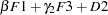
PROC CALIS can analyze matrix models of the form
 |
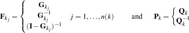
where  is a symmetric correlation or covariance matrix, each matrix
  ,
,  is the product of
  matrices
  , and each matrix
  is symmetric; that is,
 |
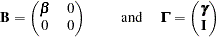
The matrices  and in the model are parameterized by the matrices
  and
and 
 |
where you can specify the type of matrix desired.
The matrices and can contain the following:
constant values
parameters to be estimated
values computed from parameters via programming statements
The parameters can be summarized in a parameter vector  . For a given covariance or correlation matrix , PROC CALIS computes the unweighted least squares (ULS), generalized least squares (GLS), maximum likelihood (ML), weighted least squares (WLS), or diagonally weighted least squares (DWLS) estimates of the vector
  .
.
Some Special Cases of the Generalized COSAN Model

Reticular Action Model—RAM (McArdle 1980; McArdle and McDonald 1984)
Structural equation model:
 |
where  is a matrix of coefficients, and
  and
and  are vectors of random variables. The variables in and can be manifest or latent variables. The endogenous variables corresponding to the components in are expressed as a linear combination of the remaining variables and a residual component in with covariance matrix
  .
.
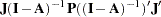
Covariance structure:
 |
with selection matrix  and
and
 |
LINEQS (Linear Equations) Model (Bentler and Weeks 1980)
Structural equation model:
 |
where  and
and  are coefficient matrices, and
  and
and  are vectors of random variables. The components of correspond to the endogenous variables; the components of correspond to the exogenous variables and to error variables. The variables in and can be manifest or latent variables. The endogenous variables in are expressed as a linear combination of the remaining endogenous variables, the exogenous variables in , and a residual component in . The coefficient matrix describes the relationships among the endogenous variables of , and
  should be nonsingular. The coefficient matrix describes the relationships between the endogenous variables of and the exogenous and error variables of .
Covariance structure:
 |
with selection matrix ,  , and
, and
 |
Keesling-Wiley-Jöreskog LISREL (Linear Structural Relationship) Model (Keesling 1972; Wiley 1973; Jöreskog 1973)
Structural equation model and measurement models:
 |
where and are vectors of latent variables (factors), and  and
and  are vectors of manifest variables. The components of correspond to endogenous latent variables; the components of correspond to exogenous latent variables. The endogenous and exogenous latent variables are connected by a system of linear equations (the structural model) with coefficient matrices
  and
and  and an error vector
  . It is assumed that matrix
  is nonsingular. The random vectors and correspond to manifest variables that are related to the latent variables and by two systems of linear equations (the measurement model) with coefficients
  and
and  and with measurement errors
  and
and  .
.
Covariance structure:
 |
 |
 |
|||
 |
|
 |
with selection matrix ,  ,
,  ,
,  , and
, and  .
.
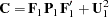

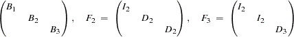
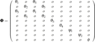
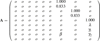
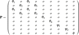
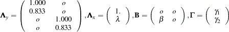
First-Order Autoregressive Longitudinal Factor Model
Example of McDonald (1980):  : Occasions of Measurement;
  : Variables (Tests);
  : Common Factors
|
|
 |
|||
 |
|
 |
|||
 |
|
 |
|||
 |
|
 |
For more information about this model, see Example 25.6.
A Structural Equation Example
This example from Wheaton et al. (1977) illustrates the relationships among the RAM, LINEQS, and LISREL models. Different structural models for these data are in Jöreskog and Sörbom (1985) and in Bentler (1985, p. 28). The data set contains covariances among six (manifest) variables collected from 932 people in rural regions of Illinois:
- Variable 1:
V1,
 : Anomie 1967
 - Variable 2:
V2,
 : Powerlessness 1967
 - Variable 3:
V3,
 : Anomie 1971
 - Variable 4:
V4,
 : Powerlessness 1971
 - Variable 5:
V5,
 : Education (years of schooling)
 - Variable 6:
V6,
 : Duncan’s Socioeconomic Index (SEI)
It is assumed that anomie and powerlessness are indicators of an alienation factor and that education and SEI are indicators for a socioeconomic status (SES) factor. Hence, the analysis contains three latent variables:
- Variable 7:
F1,
 : Alienation 1967
 - Variable 8:
F2,
 : Alienation 1971
 - Variable 9:
F3,
 : Socioeconomic Status (SES)
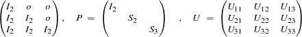
The following path diagram shows the structural model used in Bentler (1985, p. 29) and slightly modified in Jöreskog and Sörbom (1985, p. 56). In this notation for the path diagram, regression coefficients between the variables are indicated as one-headed arrows. Variances and covariances among the variables are indicated as two-headed arrows. Indicating error variances and covariances as two-headed arrows with the same source and destination (McArdle 1988; McDonald 1985) is helpful in transforming the path diagram to RAM model list input for the CALIS procedure.
Variables in Figure 25.1 are as follows:
- Variable 1:
V1,
: Anomie 1967 - Variable 2:
V2,
: Powerlessness 1967 - Variable 3:
V3,
: Anomie 1971 - Variable 4:
V4,
: Powerlessness 1971 - Variable 5:
V5,
: Education (years of schooling) - Variable 6:
V6,
: Duncan’s Socioeconomic Index (SEI) - Variable 7:
F1,
: Alienation 1967 - Variable 8:
F2,
: Alienation 1971 - Variable 9:
F3,
: Socioeconomic Status (SES)
LINEQS Model
The vector contains the six endogenous manifest variables V1, ..., V6 and the two endogenous latent variables F1 and F2. The vector contains the exogenous error variables E1, ..., E6, D1, and D2 and the exogenous latent variable F3. The path diagram corresponds to the following set of structural equations of the LINEQS model:
 |
|
 |
|||
 |
|
 |
|||
 |
|
 |
|||
 |
|
 |
|||
 |
|
 |
|||
 |
|
 |
|||
 |
|
 |
|||
 |
|
 |
This gives the matrices , , and  in the LINEQS model:
 |
 |
The LINEQS model input specification of this example for the CALIS procedure is given in the section LINEQS Model Specification.
RAM Model
The vector contains the six manifest variables  V1, ...,
  V6 and the three latent variables
  F1,
F1,  F2,
F2,  F3. The vector contains the corresponding error variables
  E1, ...,
  E6 and
  D1,
D1,  D2,
D2,  D3. The path diagram corresponds to the following set of structural equations of the RAM model:
 |
|
 |
|||
 |
|
 |
|||
 |
|
 |
|||
 |
|
 |
|||
 |
|
 |
|||
 |
|
 |
|||
 |
|
 |
|||
 |
|
 |
|||
 |
|
 |
This gives the matrices and in the RAM model:
 |
 |
The RAM model input specification of this example for the CALIS procedure is given in the section RAM Model Specification.
LISREL Model
The vector contains the four endogenous manifest variables  V1, ...,
  V4, and the vector contains the exogenous manifest variables
  V5 and
  V6. The vector contains the error variables
  E1, ...,
  E4 corresponding to
  and the vector contains the error variables
  E5 and
  E6 corresponding to . The vector contains the endogenous latent variables (factors)
  F1 and
  F2, while the vector contains the exogenous latent variable (factor)
  F3. The vector contains the errors
  D1 and
  D2 in the equations (disturbance terms) corresponding to . The path diagram corresponds to the following set of structural equations of the LISREL model:
 |
|
 |
|||
 |
|
 |
|||
 |
|
 |
|||
 |
|
 |
|||
 |
|
 |
|||
 |
|
 |
|||
 |
|
 |
|||
 |
|
 |
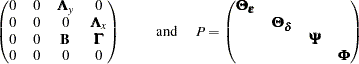
This gives the matrices  ,
,  , , , and in the LISREL model:
 |
 |
The CALIS procedure does not provide a LISREL model input specification. However, any model that can be specified by the LISREL model can also be specified by using the LINEQS, RAM, or COSAN model specifications in PROC CALIS.
Copyright © 2009 by SAS Institute Inc., Cary, NC, USA. All rights reserved.