The HPSPLIT Procedure

Example 16.6 Applying Breiman’s 1-SE Rule with Misclassification Rate
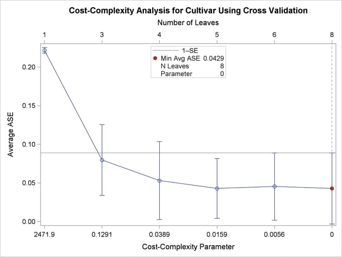
By default, the HPSPLIT procedure provides a plot for selecting the tuning parameter for cost-complexity pruning when cross validation is used to select the best subtree. The procedure selects the pruning parameter that minimizes the estimate of average square error (ASE) that is obtained by 10-fold cross validation. (See Figure 16.6 in the wine example in the section Getting Started: HPSPLIT Procedure.)
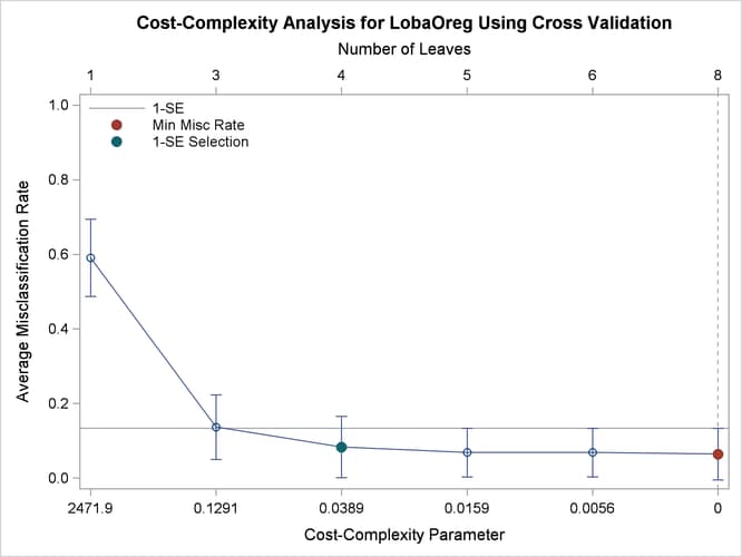
This example shows how to construct this plot by using the misclassification rate in place of the ASE and by using Breiman’s 1-SE rule to select the pruning parameter.
The following DATA step reads the wine data that are described in the section Getting Started: HPSPLIT Procedure:
data Wine;
   %let url = http://archive.ics.uci.edu/ml/machine-learning-databases;
   infile "&url/wine/wine.data" url delimiter=',';
   input Cultivar Alcohol Malic Ash Alkan Mg TotPhen
         Flav NFPhen Cyanins Color Hue ODRatio Proline;
   label Cultivar = "Cultivar"
         Alcohol  = "Alcohol"
         Malic    = "Malic Acid"
         Ash      = "Ash"
         Alkan    = "Alkalinity of Ash"
         Mg       = "Magnesium"
         TotPhen  = "Total Phenols"
         Flav     = "Flavonoids"
         NFPhen   = "Nonflavonoid Phenols"
         Cyanins  = "Proanthocyanins"
         Color    = "Color Intensity"
         Hue      = "Hue"
         ODRatio  = "OD280/OD315 of Diluted Wines"
         Proline  = "Proline";
run;
PROC HPSPLIT is run in the next step:
ods graphics on;

proc hpsplit data=Wine seed=15531 cvcc;
   ods select CrossValidationValues CrossValidationASEPlot;
   ods output CrossValidationValues=p;
   class Cultivar;
   model Cultivar = Alcohol Malic Ash Alkan Mg TotPhen Flav
                    NFPhen Cyanins Color Hue ODRatio Proline;
   grow entropy;
   prune costcomplexity;
run;
There are several differences between this step and the one in the section Getting Started: HPSPLIT Procedure:
-
The CVCC option displays a table of cost-complexity pruning based on cross validation. This table contains cross validated estimates of the misclassification rates and ASEs and their standard errors for each value of the pruning parameter.
-
An ODS SELECT statement selects only the cost-complexity pruning table and plot.
-
An ODS OUTPUT statement outputs the cost-complexity pruning table to a SAS data set.
Output 16.6.1 displays the table that you requested by using the CVCC option. Output 16.6.2 shows the default plot, which displays the ASE on the vertical axis.
Output 16.6.1: Cost-Complexity Pruning Average ASE and Misclassification Rate
| 10-Fold Cross Validation Assessment of Pruning Parameter | |||||||||||||
|---|---|---|---|---|---|---|---|---|---|---|---|---|---|
| N Leaves |
Pruning Parameter |
Average Square Error | Number of Leaves | Misclassification Rate | |||||||||
| Min | Avg | Standard Error |
Max | Min | Median | Max | Min | Avg | Standard Error |
Max | |||
| 8 | 0 | * | 0 | 0.0429 | 0.0460 | 0.1333 | 8 | 8.0 | 10 | 0.0000 | 0.0643 | 0.0690 | 0.2000 |
| 6 | 0.00562 | 0.000066 | 0.0454 | 0.0435 | 0.1333 | 5 | 6.0 | 10 | 0.0000 | 0.0684 | 0.0655 | 0.2000 | |
| 5 | 0.0159 | 0.000435 | 0.0429 | 0.0387 | 0.1193 | 5 | 5.0 | 5 | 0.0000 | 0.0684 | 0.0655 | 0.2000 | |
| 4 | 0.0389 | 0.00126 | 0.0531 | 0.0504 | 0.1344 | 3 | 4.0 | 4 | 0.0000 | 0.0831 | 0.0820 | 0.2222 | |
| 3 | 0.1291 | 0.0300 | 0.0797 | 0.0459 | 0.1623 | 3 | 3.0 | 3 | 0.0500 | 0.1368 | 0.0864 | 0.2778 | |
| 1 | 2471.9 | 0.2170 | 0.2217 | 0.00363 | 0.2288 | 1 | 1.0 | 1 | 0.3636 | 0.5908 | 0.1035 | 0.7333 | |
| * Selected pruning parameter | |||||||||||||
Output 16.6.2: Cost-Complexity Pruning Plot of Average ASE
The following steps filter the table to exclude observations that have duplicate numbers of leaves, add (subtract) the standard errors to (from) the misclassification rates, and output the information that is needed to display the reference lines, inset table, minimum misclassification rate, and 1-SE selection:
proc sort data=p;       /* Ensure MiscAverage ascends within nLeaves ties */
   by descending nleaves MiscAverage;
 run;

data plot;
   set p;
   by descending nleaves;
   if first.nleaves;                            /* Delete nLeaves dups    */
   retain yval 1e10;
   MiscMax = MiscAverage + MISCStdErr;          /* Error bar max          */
   MiscMin = MiscAverage - MISCStdErr;          /* Error bar min          */
   if MiscAverage < yval then do;
      yval = MiscAverage;                       /* Min MiscAverage        */
      call symputx('yref', MiscMax);            /* 1-SE reference line    */
      call symputx('xref', nleaves);            /* nLeaves reference line */
   end;
run;

data plot;                                      /* nLeaves at 1-SE point  */
   set plot;
   if MiscAverage <= &yref then call symputx('nleaves', nleaves);
run;

data plot;
   set plot;
   if &nleaves = nleaves then do;               /* Highlight 1-SE value   */
      xse      = nleaves;                       /* X value for 1-SE       */
      yse      = MiscAverage;                   /* Y value for 1-SE       */
   end;
   if &xref    = nleaves then do;               /* Highlight minimum      */
      xmin     = nleaves;                       /* X value for minimum    */
      ymin     = MiscAverage;                   /* Y value for minimum    */
   end;
   format pruningparameter best6.;              /* X axis format          */
run;
These steps create several macro and DATA step variables. The number of leaves that are selected by using the 1-SE rule is
saved in the macro variable nLeaves. You can use PROC SGPLOT along with these new variables as follows to create the cost-complexity pruning plot with the misclassification
rate on the vertical axis:
proc sgplot noautolegend;
   title 'Cost-Complexity Analysis for LobaOreg Using Cross Validation';
   refline &xref / axis=x2 lineattrs=(pattern=shortdash);
   refline &yref / axis=y  name='a' legendlabel='1-SE';
   series  y=MiscAverage x=nleaves / x2axis lineattrs=graphdata1;
   scatter y=MiscAverage x=pruningparameter / yerrorlower=MiscMin
                         yerrorupper=MiscMax errorbarattrs=graphdata1;
   scatter y=ymin x=xmin / markerattrs=GraphData2(symbol=circlefilled size=9px)
                           x2axis name='b' legendlabel='Min Misc Rate';
   scatter y=yse  x=xse  / markerattrs=GraphData3(symbol=circlefilled size=9px)
                           x2axis name='c' legendlabel='1-SE Selection';
   xaxis   type=discrete label='Cost-Complexity Parameter' reverse;
   x2axis  type=discrete label='Number of Leaves';
   yaxis   label='Average Misclassification Rate' min=0 max=1;
   keylegend 'a' 'b' 'c' / location=inside across=1 noborder;
run;
Output 16.6.3 displays the results.
Output 16.6.3: Cost-Complexity Analysis Based on Misclassification Rate
You can rerun the analysis and use the selected number of leaves by specifying the nLeaves macro variable in the PRUNE statement as follows:
proc hpsplit data=Wine seed=15531;
   class Cultivar;
   model Cultivar = Alcohol Malic Ash Alkan Mg TotPhen Flav
                    NFPhen Cyanins Color Hue ODRatio Proline;
   prune costcomplexity(leaves=&nLeaves);
run;
The results of this step are not displayed.