The HPLMIXED Procedure

ML and REML methods provide estimates of ![]() and
and ![]() , which are denoted
, which are denoted ![]() and
and ![]() , respectively. To obtain estimates of
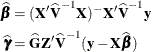
, respectively. To obtain estimates of ![]() and predicted values of
and predicted values of ![]() , the standard method is to solve the mixed model equations (Henderson, 1984):
, the standard method is to solve the mixed model equations (Henderson, 1984):
The solutions can also be written as
and have connections with empirical Bayes estimators (Laird and Ware, 1982; Carlin and Louis, 1996). Note that the ![]() are random variables and not parameters (unknown constants) in the model. Technically, determining values for
are random variables and not parameters (unknown constants) in the model. Technically, determining values for ![]() from the data is thus a prediction task, whereas determining values for
from the data is thus a prediction task, whereas determining values for ![]() is an estimation task.
is an estimation task.
The mixed model equations are extended normal equations. The preceding expression assumes that ![]() is nonsingular. For the extreme case where the eigenvalues of
is nonsingular. For the extreme case where the eigenvalues of ![]() are very large,
are very large, ![]() contributes very little to the equations and
contributes very little to the equations and ![]() is close to what it would be if
is close to what it would be if ![]() actually contained fixed-effects parameters. On the other hand, when the eigenvalues of
actually contained fixed-effects parameters. On the other hand, when the eigenvalues of ![]() are very small,
are very small, ![]() dominates the equations and
dominates the equations and ![]() is close to
is close to ![]() . For intermediate cases,
. For intermediate cases, ![]() can be viewed as shrinking the fixed-effects estimates of
can be viewed as shrinking the fixed-effects estimates of ![]() toward
toward ![]() (Robinson, 1991).
(Robinson, 1991).
If ![]() is singular, then the mixed model equations are modified (Henderson, 1984) as follows:
is singular, then the mixed model equations are modified (Henderson, 1984) as follows:
Denote the generalized inverses of the nonsingular ![]() and singular
and singular ![]() forms of the mixed model equations by
forms of the mixed model equations by ![]() and
and ![]() , respectively. In the nonsingular case, the solution
, respectively. In the nonsingular case, the solution ![]() estimates the random effects directly. But in the singular case, the estimates of random effects are achieved through a back-transformation
estimates the random effects directly. But in the singular case, the estimates of random effects are achieved through a back-transformation
![]() where
where ![]() is the solution to the modified mixed model equations. Similarly, while in the nonsingular case
is the solution to the modified mixed model equations. Similarly, while in the nonsingular case ![]() itself is the estimated covariance matrix for
itself is the estimated covariance matrix for ![]() , in the singular case the covariance estimate for
, in the singular case the covariance estimate for ![]() is given by
is given by ![]() where
where
An example of when the singular form of the equations is necessary is when a variance component estimate falls on the boundary
constraint of ![]() .
.