Nonparametric Kernel Smoother

Fit Analyses

Nonparametric Kernel Smoother

A kernel estimator uses an explicitly defined set of weights at each point x to produce the estimate at x. The kernel estimator of f has the form

$\hat{f_\lambda}(x) = \sum_{i=1}^n{W( x , x_{i} ; \lambda) y_{i}}$

where W ${( x , x_{i} ; \lambda)}$ is the weight function that depends on the smoothing parameter $\lambda$ .

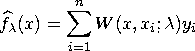
The weights are derived from a single function that is independent of the design

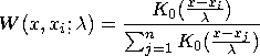
$W( x , x_{i} ; \lambda) = \frac{K_{0} ( \frac{x- x_{i}}{\lambda} )}{\sum_{j=1}^n{K_{0} ( \frac{x- x_{j}}{\lambda} ) }}$

where K₀ is a kernel function and $\lambda$ is the bandwidth or smoothing parameter. The weights are nonnegative and sum to 1.

Symmetric probability density functions commonly used as kernel functions are

$\bullet Normal$	$K_{0}(t) = \frac{1}{\sqrt{2{\pi}}} \exp( - t^2/2 )$	for $-\infty\lt t\lt\infty$
$\bullet Triangular$	$K_{0}(t) = \{ 1 - {\| t\|} \ 0 \ .$	${for \| t\|\le 1} \ {otherwise} \$
$\bullet Quadratic$	$K_{0}(t) = \{ \frac{3}4 (1 - t^2) \ 0 \ .$	${for \| t\|\le 1} \ {otherwise} \$

You select a bandwidth $\lambda$ for each kernel estimator by specifying c in the formula

$\lambda = n^{-\frac{1}5} Q c$

where Q is the sample interquartile range of the explanatory variable and n is the sample size. This formulation makes c independent of the units of X.

SAS/INSIGHT software divides the range of the explanatory variable into 128 evenly spaced intervals, then approximates the data on this grid and uses the fast Fourier transformation (Silverman 1986) to estimate the kernel fit on this grid. For a data point x_i that lies between two grid points, a linear interpolation is used to compute the predicted value. A small value of $\lambda$ (relative to the width of the interval) may give unstable estimates of the kernel fit.

After choosing Curves:Kernel, you specify a kernel and smoothing parameter selection method in the Kernel Fit dialog.

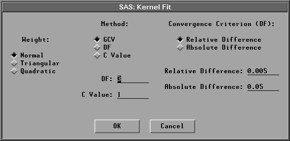
Figure 39.42: Kernel Fit Dialog

The default Weight:Normal uses a normal weight, and Method:GCV uses a c value that minimizes ${ \rm{MSE}_{GCV}(\lambda)}$ .Figure 39.43 illustrates normal kernel estimates with c values of 0.0944 (the GCV value) and 0.7546 (DF=3). Use the slider to change the c value of the kernel fit.

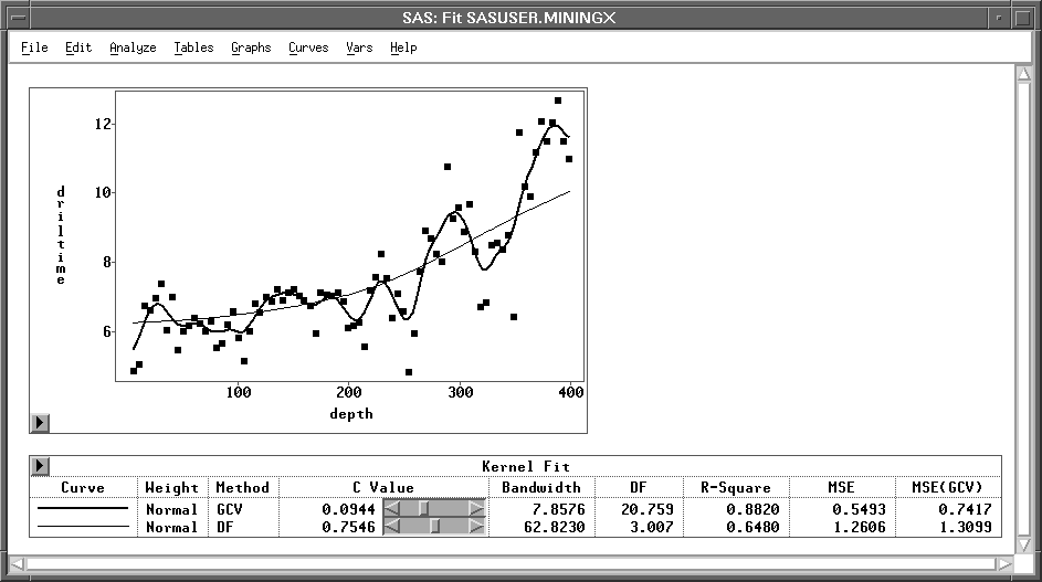
Figure 39.43: Kernel Estimates

Top of Page