Nonparametric Local Polynomial Smoother

Fit Analyses

Nonparametric Local Polynomial Smoother

The kernel estimator fits a local mean at each point x and thus cannot even estimate a line without bias (Cleveland, Cleveland, Devlin and Grosse 1988). An estimator based on locally-weighted regression lines or locally-weighted quadratic polynomials may give more satisfactory results.

A local polynomial smoother fits a locally-weighted regression at each point x to produce the estimate at x. Different types of regression and weight functions are used in the estimation.

SAS/INSIGHT software provides the following three types of regression:

$\bullet Mean$		a locally-weighted mean
$\bullet Linear$		a locally-weighted regression line
$\bullet Quadratic$		a locally-weighted quadratic polynomial regression

The weights are derived from a single function that is independent of the design

$W( x , x_{i} ; \lambda_{i}) = K_{0} ( \frac{x- x_{i}}{\lambda_{i}} )$

where K₀ is a weight function and ${ \lambda_{i}}$ is the local bandwidth at x_i.

SAS/INSIGHT software uses the following weight functions:

$\bullet Normal$	$K_{0}(t) = \{ \exp( - t^2/2 ) \ 0 \ .$	${for \| t\|\le 3.5} \ {otherwise} \$
$\bullet Triangular$	$K_{0}(t) = \{ 1 - {\| t\|} \ 0 \ .$	${for \| t\|\le 1} \ {otherwise} \$
$\bullet Quadratic$	$K_{0}(t) = \{ 1 - t^2 \ 0 \ .$	${for \| t\|\le 1} \ {otherwise} \$
$\bullet Tri-Cube$	$K_{0}(t) = \{ (1 - \| t\|^3)^3 \ 0 \ .$	${for \| t\|\le 1} \ {otherwise} \$

Note	The normal weight function is proportional to a truncated normal density function.

SAS/INSIGHT software provides two methods to compute the local bandwidth ${ \lambda_{i}}$ .The loess estimator (Cleveland 1979; Cleveland, Devlin and Grosse 1988) evaluates ${ \lambda_{i}}$ based on the furthest distance from k nearest neighbors. A fixed bandwidth local polynomial estimator uses a constant bandwidth $\lambda$ at each x_i.

For a loess estimator, you select k nearest neighbors by specifying a positive constant $\alpha$ .For $\alpha\le 1$ , k is $\alpha n$ truncated to an integer, where n is the number of observations. For $\alpha\gt 1$ , k is set to n.

The local bandwidth ${ \lambda_{i}}$ is then computed as

$\lambda_{i} = \{ d_{(k)}( x_{i}) & {for 0 \lt \alpha \le 1} \ \alpha d_{(n)}( x_{i}) & {for \alpha \gt 1} \ .$

where d_(k)( x_i) is the furthest distance from x_i to its k nearest neighbors.

Note	For $\alpha\le 1$ , the local bandwidth ${ \lambda_{i}}$ is a function of k and thus a step function of $\alpha$ .

For a fixed bandwidth local polynomial estimator, you select a bandwidth $\lambda$ by specifying c in the formula

$\lambda = n^{-\frac{1}5} Q c$

where Q is the sample interquartile range of the explanatory variable and n is the sample size. This formulation makes c independent of the units of X.

Note	A fixed bandwidth local mean estimator is equivalent to a kernel smoother.

By default, SAS/INSIGHT software divides the range of the explanatory variable into 128 evenly spaced intervals, then it fits locally-weighted regressions on this grid. A small value of c or $\alpha$ may give the local polynomial fit to the data points near the grid points only and may not apply to the remaining points.

For a data point x_i that lies between two grid points ${ x_{i[j]}\le x_{i}\lt x_{i[j+1]}}$ , the predicted value is the weighted average of the two predicted values at the two nearest grid points:

$(1- d_{ij}) \hat{ y_{i}}_{[j]} + d_{ij} \hat{ y_{i}}_{[j+1]}$

where $\hat{ y_{i}}_{[j]}$ and $\hat{ y_{i}}_{[j+1]}$ are the predicted values at the two nearest grid points and

d_ij = [(x_i- x_i[j])/(x_i[j+1]- x_i[j] )]

A similar algorithm is used to compute the degrees of freedom of a local polynomial estimate, ${ df_{\lambda}}$ = trace( $H_{\lambda}$ ). The ith diagonal element of the matrix $H_{\lambda}$ is

(1- d_ij) h_i[j] + d_ij h_i[j+1]

where h_i[j] and h_i[j+1] are the ith diagonal elements of the projection matrices of the two regression fits.

After choosing Curves:Loess from the menu, you specify a loess fit in the Loess Fit dialog.

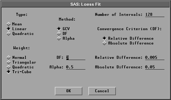
Figure 39.44: Loess Fit Dialog

In the dialog, you can specify the number of intervals, the regression type, the weight function, and the method for choosing the smoothing parameter. The default Type:Linear uses a linear regression, Weight:Tri-Cube uses a tri-cube weight function, and Method:GCV uses an $\alpha$ value that minimizes ${ \rm{MSE}_{GCV}(\lambda)}$ .

Figure 39.45 illustrates loess estimates with Type=Linear, Weight=Tri-Cube, and $\alpha$ values of 0.0930 (the GCV value) and 0.7795 (DF=3). Use the slider to change the $\alpha$ value of the loess fit.

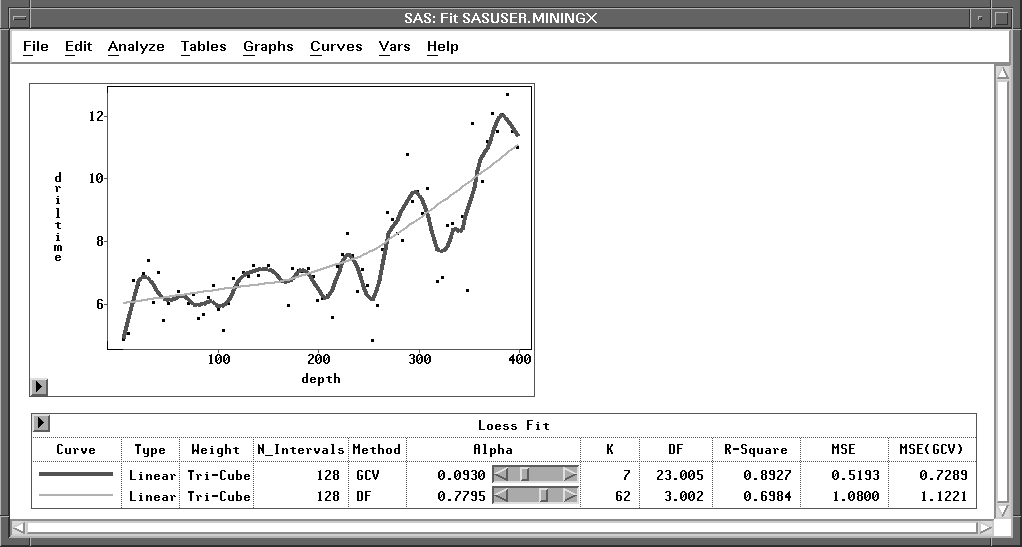
Figure 39.45: Loess Estimates

The loess degrees of freedom is a function of local bandwidth ${ \lambda_{i}}$ .For $\alpha\le 1$ , ${ \lambda_{i}}$ is a step function of $\alpha$ and thus the loess df is a step function of $\alpha$ .The convergence criterion applies only when the specified df is less than ${df}_{(\alpha=1)}$ ,the loess df for $\alpha=1$ .When the specified df is greater than ${df}_{(\alpha=1)}$ , SAS/INSIGHT software uses the $\alpha$ value that has its df closest to the specified df.

Similarly, you can choose Curves:Local Polynomial, Fixed Bandwidth from the menu to specify a fixed bandwidth local polynomial fit.

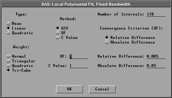
Figure 39.46: Fixed Bandwidth Local Polynomial Fit Dialog

Figure 39.47 illustrates fixed bandwidth local polynomial estimates with Type=Linear, Weight=Tri-Cube, and c values of 0.2026 (the GCV value) and 2.6505 (DF=3). Use the slider to change the c value of the local polynomial fit.

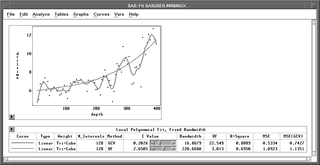
Figure 39.47: Fixed Bandwidth Local Polynomial Estimates

Top of Page