Kernel Surface Plot

Fit Analyses

Kernel Surface Plot

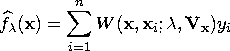
A kernel estimator uses an explicitly defined set of weights at each point x to produce the estimate at x. The kernel estimator of f has the form

$\hat{f_\lambda}(x) = \sum_{i=1}^n{W( x , x_{i}; \lambda, V_{x}) y_{i}}$

where W ${( x , x_{i}; \lambda, V_{x})}$ is the weight function that depends on the smoothing parameter $\lambda$ and the diagonal matrix V_x of the squares of the sample interquartile ranges.

The weights are derived from a single function that is independent of the design

$W( x , x_{i}; \lambda, V_{x}) = \frac{K_{0} ( (x - x_{i})/\lambda, V_{x} )}{\sum_{j=1}^n{K_{0} ( (x - x_{j})/\lambda, V_{x} ) } }$

where K₀ is a kernel function and $\lambda$ is the bandwidth or smoothing parameter. The weights are nonnegative and sum to 1.

Symmetric probability density functions commonly used as kernel functions are

$\bullet Normal$	$K_{0}(t, V) = \frac{1}{2{\pi}} \exp( - \frac{1}2 {t'} V^{-1} t)$	for all t
$\bullet Quadratic$	$K_{0}(t, V) = \{ \frac{2}{{\pi}} (1-{t'} V^{-1} t) \ 0 \ .$	${for {t'} V^{-1} t \le 1} \ {otherwise} \$
$\bullet Biweight$	$K_{0}(t, V) = \{ \frac{3}{{\pi}} (1-{t'} V^{-1} t)^2 \ 0 \ .$	${for {t'} V^{-1} t \le 1} \ {otherwise} \$
$\bullet Triweight$	$K_{0}(t, V) = \{ \frac{4}{{\pi}} (1-{t'} V^{-1} t)^3 \ 0 \ .$	${for {t'} V^{-1} t \le 1} \ {otherwise} \$

You select a bandwidth $\lambda$ for each kernel estimator by specifying c in the formula

$\lambda = n^{-\frac{1}6} c$

where n is the sample size. Both $\lambda$ and c are independent of the units of X.

SAS/INSIGHT software divides the range of each explanatory variable into a number of evenly spaced intervals, then estimates the kernel fit on this grid. For a data point x_i that lies between two grid points, a linear interpolation is used to compute the predicted value. For x_i that lies inside a square of grid points, a pair of points that lie on the same vertical line as x_i and each lying between two grid points can be found. A linear interpolation of these two points is used to compute the predicted value.

After choosing Graphs:Surface Plot:Kernel from the menu, you specify a kernel and smoothing parameter selection method in the Kernel Fit dialog.

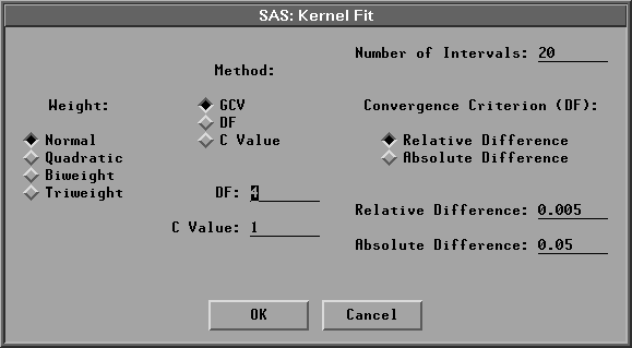
Figure 39.30: Kernel Surface Fit Dialog

By default, SAS/INSIGHT software divides the range of each explanatory variable into 20 evenly spaced intervals, uses a normal weight, and uses a c value that minimizes ${ \rm{MSE}_{GCV}(\lambda)}$ .Figure 39.31 illustrates normal kernel estimates with c values of 0.5435 (the GCV value) and 1.0. Use the slider to change the c value of the kernel fit.

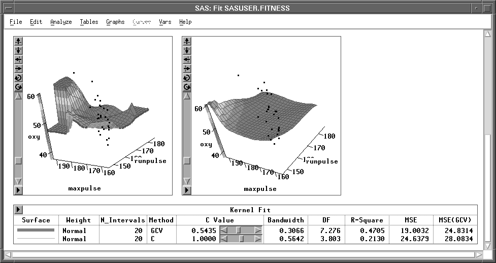
Figure 39.31: Kernel Surface Plot

Top of Page