Smoothing Spline Surface Plot

Fit Analyses

Smoothing Spline Surface Plot

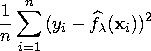
Two criteria can be used to select an estimator ${\hat{f_\lambda}}$ for the function f:

goodness of fit to the data
smoothness of the fit

A standard measure of goodness of fit is the mean residual sum of squares

$\frac{1}n\sum_{i=1}^n{( y_{i}- \hat{f_\lambda}( x_{i}))^2}$

A measure of the smoothness of a fit is an integrated squared second derivative

$J_{2} ( f_{\lambda}) = \int_{-{\infty}}^{{\infty}}{\int_{-{\infty}}^{{\infty}}{... ... \frac{\partial^2 f_{\lambda}}{\partial x_{2}^2 } )^2 ) d x_{1} } d x_{2} }$

A single criterion that combines the two criteria is then given by

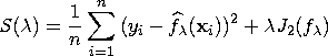
$S(\lambda) = \frac{1}n \sum_{i=1}^n{( y_{i}- \hat{f_\lambda}( x_{i}))^2} + \lambda J_{2} ( f_{\lambda})$

where ${\hat{f_\lambda}}$ belongs to the set of all continuously differentiable functions with square integrable second derivatives, and $\lambda$ is a positive constant.

The estimator that results from minimizing S( $\lambda$ )is called a thin-plate smoothing spline estimator. Wahba and Wendelberger (1980) derived a closed form expression for the thin-plate smoothing spline estimator.

Note	The computations for a thin-plate smoothing spline are time intensive, especially for large data sets.

The smoothing parameter $\lambda$ controls the amount of smoothing; that is, it controls the trade-off between the goodness of fit to the data and the smoothness of the fit. You select a smoothing parameter $\lambda$ by specifying a constant c in the formula

$\lambda = c / 100$

The values of the explanatory variables are scaled by their corresponding interquartile ranges before the computations. This makes the computations independent of the units of X₁ and X₂.

After choosing Graphs:Surface Plot:Spline from the menu, you specify a smoothing parameter selection method in the Spline Fit dialog.

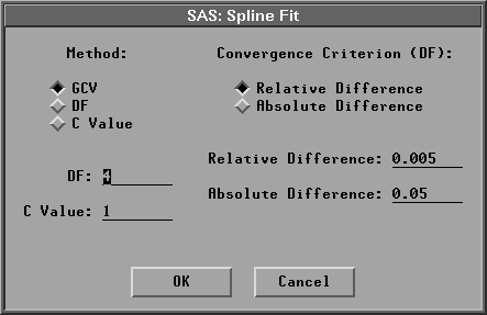
Figure 39.28: Spline Surface Fit Dialog

The default Method:GCV uses a c value that minimizes the generalized cross validation mean squared error ${ \rm{MSE}_{GCV}(\lambda)}$ .Figure 39.29 displays smoothing spline estimates with c values of 0.0000831 (the GCV value) and 0.4127 (DF=6). Use the slider in the table to change the c value of the spline fit.

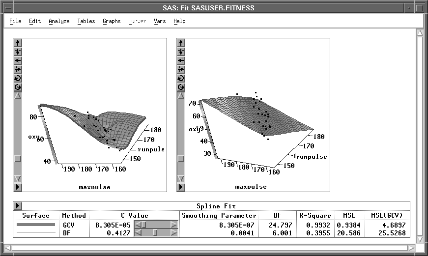
Figure 39.29: Smoothing Spline Surface Plot

Top of Page