Examining Distributions

Testing Distributions

You can add a graph to examine the cumulative distribution function, and you can test for distributions by using the Kolmogorov statistic.

Choose Curves:CDF Confidence Band:95%.

[menu]
Figure 12.19: Confidence Band Menu

This adds a graph of the cumulative distribution function with 95% confidence bands, as illustrated in Figure 12.20.

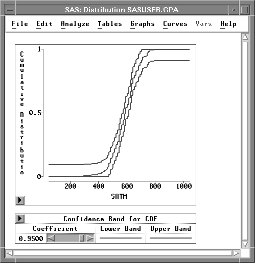
Figure 12.20: Cumulative Distribution Function

Choose Curves:Test for Distribution.

This displays the test for distribution dialog. The default settings test whether the data are from a normal distribution.

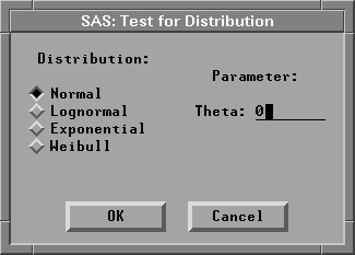
Figure 12.21: Test for Distribution Dialog

Click OK in the dialog.

This adds a curve to the graph and a Test for Distribution table to the window, as illustrated in Figure 12.22.

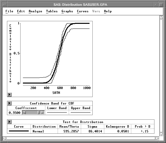
Figure 12.22: Test for Normal Distribution

The smooth curve in the graph represents the fitted normal distribution. It lies quite close to the irregular curve representing the empirical distribution function. The Test for Distribution table contains the mean (Mean / Theta) and standard deviation (Sigma) for the data along with the results of Kolmogorov's test for normality. This tests the null hypothesis that the data come from a normal distribution with unknown mean and variance. The p-value (Prob > D), also referred to as the probability value or observed significance level, is the probability of obtaining a D statistic greater than the computed D statistic when the null hypothesis is true. The smaller the p-value, the stronger the evidence against the null hypothesis. The computed p-value is large (>0.15), so there is no reason to conclude that these data are not normally distributed.