Kernel Density

Distribution Analyses

Kernel Density

Kernel density estimation provides normal, triangular, and quadratic kernel density estimators. The general form of a kernel estimator is

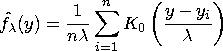
$\hat{ f_{\lambda}}(y) = \frac{1}{n \lambda} \sum_{i=1}^n K_0(\frac{y- y_{i}}{\lambda})$

where K₀ is a kernel function and $\lambda$ is the bandwidth.

Some symmetric probability density functions commonly used as kernel functions are

$\bullet Normal$	$K_0(t) = \frac{1}{\sqrt{2{\pi}}} \exp( - t^2/2 )$	for $-\infty\lt t\lt\infty$
$\bullet Triangular$	$K_0(t) = \{ 1 - {\| t\|} \ 0 \ .$	${for \| t\|\le 1} \ {otherwise} \$
$\bullet Quadratic$	$K_0(t) = \{ \frac{3}4 (1 - t^2) \ 0 \ .$	${for \| t\|\le 1} \ {otherwise} \$

Both theory and practice suggest that the choice of a kernel function is not crucial to the statistical performance of the method (Epanechnikov 1969). With a specific kernel function, the value of $\lambda$ determines the degree of averaging in the estimate of the density function and is called a smoothing parameter. You select a bandwidth $\lambda$ for each kernel estimator by specifying c in the formula

$\lambda = n^{-\frac{1}5} Q c$

where Q is the sample interquartile range of the Y variable. This formulation makes c independent of the units of Y.

For a specific kernel function, the discrepancy between the density estimator ${\hat{ f_{\lambda}}(y)}$ and the true density f(y) can be measured by the mean integrated square error

$\rm{MISE}(\lambda) = \int_{y}^{}{\{E(\hat{ f_{\lambda}}(y)) - f(y)\}^2dy } + \int_{y}^{}{\rm{Var}(\hat{ f_{\lambda}}(y)) \,dy }$

which is the sum of the integrated square bias and the integrated variance.

An approximate mean integrated square error based on the bandwidth $\lambda$ is

$\rm{AMISE}(\lambda) = \frac{1}4 \lambda^4 ( \int_{t}^{}{t^2K(t)dt} )^2 \int_{y}^{}{({f"}(y))^2\,dy } + \frac{1}{n\lambda} \int_{t}^{}{K(t)^2 dt }$

If f(y) is assumed normal, then a bandwidth based on the sample mean and variance can be computed to minimize AMISE. The resulting bandwidth for a specific kernel is used when the associated kernel function is selected in the density estimation options dialog. This is equivalent to choosing MISE from the normal, triangular, or quadratic kernel menus. If f(y) is not roughly normal, this choice may not be appropriate.

SAS/INSIGHT software divides the range of the data into 128 evenly spaced intervals, then approximates the data on this grid and uses the fast Fourier transformation (Silverman 1986) to estimate the density.

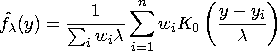
If you select a Weight variable, the kernel estimator is modified to include the individual observation weights.

$\hat{ f_{\lambda}} (y) = \frac{1}{\sum_{i}^{}{w_{i}} \lambda } \sum_{i=1}^n w_{i} K_0(\frac{y- y_{i}}{\lambda})$

You can specify the kernel function in the density estimation options dialog or from the Curves menu. When you specify the kernel function in the density estimation options dialog, AMISE is used. After choosing Curves:Kernel Density from the menu, you can specify the kernel function and use either AMISE or a specified C value in the Kernel Density Estimation dialog.

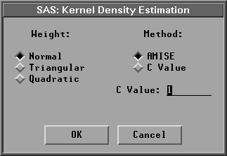
Figure 38.25: Kernel Density Dialog

The default uses a normal kernel density with a c value that minimizes the AMISE. Figure 38.26 displays normal kernel estimates with c = 0.7852 (the AMISE value) and c = 0.25. Small values of c (and hence small values of the smoothing parameter $\lambda$ ) provide jagged estimates as the curve more closely follows the data points. Large values of c provide smoother estimates. The Mode is the point with the largest estimated density. Use the slider to change the smoothing parameter, c.

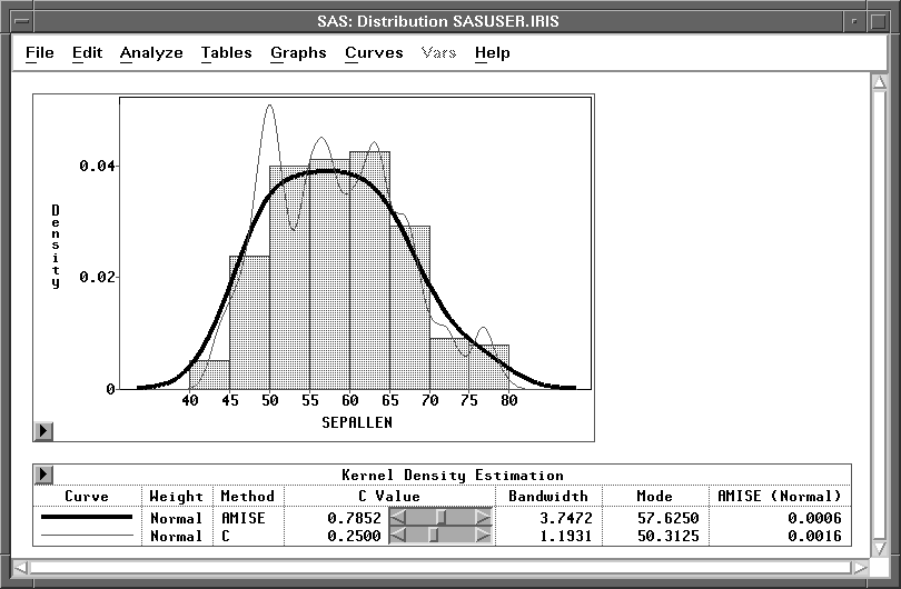
Figure 38.26: Kernel Density Estimation

Top of Page