XCHART Statement: CUSUM Procedure
- Overview
-
Getting Started

-
Syntax
-
Details
Basic Notation for Cusum Charts Formulas for Cumulative Sums Defining the Decision Interval for a One-Sided Cusum Scheme Defining the V-Mask for a Two-Sided Cusum Scheme Designing a Cusum Scheme Cusum Charts Compared with Shewhart Charts Methods for Estimating the Standard Deviation Output Data Sets ODS Tables ODS Graphics Input Data Sets Missing Values
-
Examples
Creating a One-Sided Cusum Chart with a Decision Interval
[See CUSONES1 in the SAS/QC Sample Library]An alternative to the V-mask cusum chart is the one-sided cusum chart with a decision interval, which is sometimes referred to as the "computational form of the cusum chart." This example illustrates how you can create a one-sided cusum chart for individual measurements.
A can of oil is selected every hour for fifteen hours. The cans are weighed, and their weights are saved in a SAS data set named Cans:1
data Cans;
   length comment $16;
   label Hour = 'Hour';
   input Hour Weight comment $16. ;
datalines;
 1  8.024
 2  7.971
 3  8.125
 4  8.123
 5  8.068
 6  8.177  Pump Adjusted
 7  8.229  Pump Adjusted
 8  8.072
 9  8.066
10  8.089
11  8.058
12  8.147
13  8.141
14  8.047
15  8.125
;
Suppose the problem is to detect a positive shift in the process mean of one standard deviation ( ) from the target of 8.100 ounces. Furthermore, suppose that
a known value
 is available for the process standard deviation
 an in-control average run length (ARL) of approximately 100 is required
an ARL of approximately five is appropriate for detecting the shift
Table 6.3 indicates that these ARLs can be achieved with the decision interval  and the reference value
  . The following statements use these parameters to create the chart and tabulate the cusum scheme:
options nogstyle;
goptions ftext=swiss;
symbol v=dot color=salmon h=1.8 pct;
title "One-Sided Cusum Analysis";
proc cusum data=Cans;
   xchart Weight*Hour /
      mu0      = 8.100     /* target mean for process     */
      sigma0   = 0.050     /* known standard deviation    */
      delta    = 1         /* shift to be detected        */
      h        = 3         /* cusum parameter h           */
      k        = 0.5       /* cusum parameter k           */
      scheme   = onesided  /* one-sided decision interval */
      tableall             /* table                       */
      cinfill  = ywh
      cframe   = bigb
      cout     = salmon
      cconnect = salmon
      climits  = black
      coutfill = bilg;
   label Weight = 'Cusum of Weight';
run;
options gstyle;
The NOGSTYLE system option causes ODS styles not to affect traditional graphics. Instead, the SYMBOL statement, GOPTIONS, and XCHART statement options control the appearance of the graph. The GSTYLE system option restores the use of ODS styles for traditional graphics produced subsequently. The chart is shown in Figure 6.6.
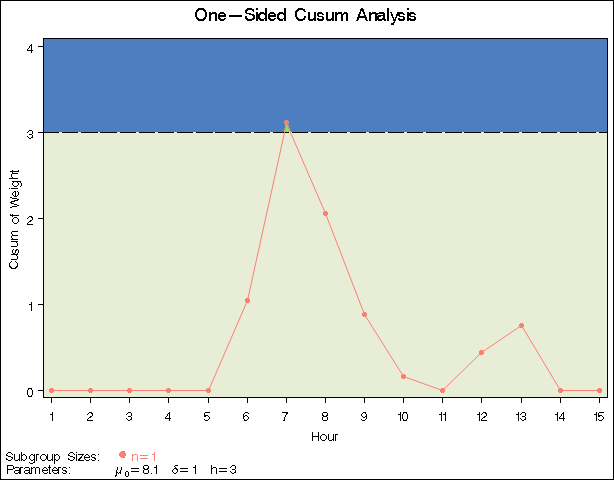
The cusum plotted at Hour=t is
 |
where  , and
, and  is the standardized deviation of the
  th measurement from the target.
 |
The cusum  is referred to as an upper cumulative sum. A shift is signaled at the seventh hour since
  exceeds
  . For further details, see One-Sided Cusum Schemes.
The option TABLEALL requests the tables shown in Figure 6.7, Figure 6.8, and Figure 6.9. The table in Figure 6.7 summarizes the cusum scheme, and it confirms that an in-control ARL of 117.6 and an ARL of 6.4 at are achieved with the specified and  .
.
| Cusum Parameters | |
|---|---|
| Process Variable | Weight (Cusum of Weight) |
| Subgroup Variable | Hour (Hour) |
| Scheme | One-Sided |
| Target Mean (Mu0) | 8.1 |
| Sigma0 | 0.05 |
| Delta | 1 |
| Nominal Sample Size | 1 |
| h | 3 |
| k | 0.5 |
| Average Run Length (Delta) | 6.40390895 |
| Average Run Length (0) | 117.595692 |
The table in Figure 6.8 tabulates the information displayed in Figure 6.6.
| One-Sided Cusum Analysis |
| Cumulative Sum Chart Summary for Weight | |||||
|---|---|---|---|---|---|
| Hour | Subgroup Sample Size |
Individual Value |
Cusum | Decision Interval |
Decision Interval Exceeded |
| 1 | 1 | 8.0240000 | 0.0000000 | 3.0000 | |
| 2 | 1 | 7.9710000 | 0.0000000 | 3.0000 | |
| 3 | 1 | 8.1250000 | 0.0000000 | 3.0000 | |
| 4 | 1 | 8.1230000 | 0.0000000 | 3.0000 | |
| 5 | 1 | 8.0680000 | 0.0000000 | 3.0000 | |
| 6 | 1 | 8.1770000 | 1.0400000 | 3.0000 | |
| 7 | 1 | 8.2290000 | 3.1200000 | 3.0000 | Upper |
| 8 | 1 | 8.0720000 | 2.0600000 | 3.0000 | |
| 9 | 1 | 8.0660000 | 0.8800000 | 3.0000 | |
| 10 | 1 | 8.0890000 | 0.1600000 | 3.0000 | |
| 11 | 1 | 8.0580000 | 0.0000000 | 3.0000 | |
| 12 | 1 | 8.1470000 | 0.4400000 | 3.0000 | |
| 13 | 1 | 8.1410000 | 0.7600000 | 3.0000 | |
| 14 | 1 | 8.0470000 | 0.0000000 | 3.0000 | |
| 15 | 1 | 8.1250000 | 0.0000000 | 3.0000 | |
The table in Figure 6.9 presents the computational form of the cusum scheme described by Lucas (1976).
| One-Sided Cusum Analysis |
| Computational Cumulative Sum for Weight | ||||
|---|---|---|---|---|
| Hour | Subgroup Sample Size |
Individual Value |
Upper Cusum |
Number of Consecutive Upper Sums > 0 |
| 1 | 1 | 8.0240000 | 0.0000000 | 0 |
| 2 | 1 | 7.9710000 | 0.0000000 | 0 |
| 3 | 1 | 8.1250000 | 0.0000000 | 0 |
| 4 | 1 | 8.1230000 | 0.0000000 | 0 |
| 5 | 1 | 8.0680000 | 0.0000000 | 0 |
| 6 | 1 | 8.1770000 | 1.0400000 | 1 |
| 7 | 1 | 8.2290000 | 3.1200000 | 2 |
| 8 | 1 | 8.0720000 | 2.0600000 | 3 |
| 9 | 1 | 8.0660000 | 0.8800000 | 4 |
| 10 | 1 | 8.0890000 | 0.1600000 | 5 |
| 11 | 1 | 8.0580000 | 0.0000000 | 0 |
| 12 | 1 | 8.1470000 | 0.4400000 | 1 |
| 13 | 1 | 8.1410000 | 0.7600000 | 2 |
| 14 | 1 | 8.0470000 | 0.0000000 | 0 |
| 15 | 1 | 8.1250000 | 0.0000000 | 0 |
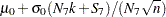
Following the method of Lucas (1976), the process average at the out-of-control point (Hour=7) can be estimated as
 |
|||||
 |
|
 |
|||
|
|
 |
|||
where  is the upper sum at Hour=7, and
  is the number of successive positive upper sums at Hour=7.