QQPLOT Statement: CAPABILITY Procedure

Three-Parameter Lognormal Plots

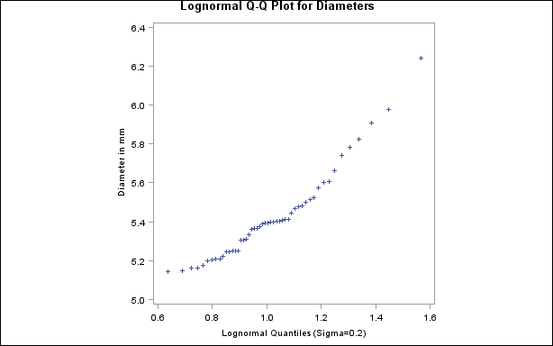
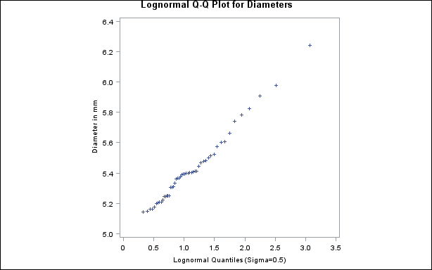
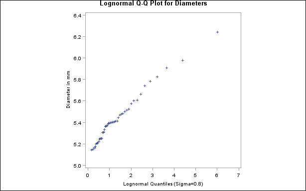
[See CAPQQ2 in the SAS/QC Sample Library]The three-parameter lognormal distribution depends on a threshold parameter , a scale parameter , and a shape parameter . You can estimate from a series of lognormal Q-Q plots with different values of . The estimate is the value of that linearizes the point pattern. You can then estimate the threshold and scale parameters from the intercept and slope of the point pattern. The following statements create the series of plots in Output 5.22.1 through Output 5.22.3 for values of 0.2, 0.5, and 0.8:

ods graphics off;
symbol v=plus;
title 'Lognormal Q-Q Plot for Diameters';
proc capability data=Measures noprint;
   qqplot Diameter / lognormal(sigma=0.2 0.5 0.8)
                     square;
run;

Output 5.22.1 Lognormal Quantile-Quantile Plot ( =0.2)

Output 5.22.2 Lognormal Quantile-Quantile Plot ( =0.5)

Output 5.22.3 Lognormal Quantile-Quantile Plot ( =0.8)

Note: You must specify a value for the shape parameter for a lognormal Q-Q plot with the SIGMA= option or its alias, the SHAPE= option.

The plot in Output 5.22.2 displays the most linear point pattern, indicating that the lognormal distribution with provides a reasonable fit for the data distribution.

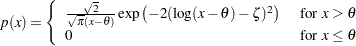
Data with this particular lognormal distribution have the density function

The points in the plot fall on or near the line with intercept and slope . Based on Output 5.22.2, and 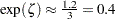, giving .

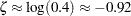Estimating Percentiles

[See CAPQQ2 in the SAS/QC Sample Library]You can use a Q-Q plot to estimate percentiles such as the th percentile of the lognormal distribution.¹

The point pattern in Output 5.22.2 has a slope of approximately 0.39 and an intercept of 5. The following statements reproduce this plot, adding a lognormal reference line with this slope and intercept.

ods graphics on;
title 'Lognormal Q-Q Plot for Diameters';
proc capability data=Measures noprint;
   qqplot Diameter / lognormal(sigma=0.5 theta=5 slope=0.39)
                     pctlaxis(grid)
                     vref  = 5.8 5.9 6.0;
run;

The ODS GRAPHICS ON statement specified before the PROC CAPABILITY statement enables ODS Graphics, so the Q-Q plot is created using ODS Graphics instead of traditional graphics. The result is shown in Output 5.22.4.

Output 5.22.4 Lognormal Q-Q Plot Identifying Percentiles

The PCTLAXIS option labels the major percentiles, and the GRID option draws percentile axis reference lines. The th percentile is 5.9, since the intersection of the distribution reference line and the th reference line occurs at this value on the vertical axis.

Alternatively, you can compute this percentile from the estimated lognormal parameters. The th percentile of the lognormal distribution is

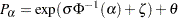where is the inverse cumulative standard normal distribution. Consequently,

Two-Parameter Lognormal Plots

[See CAPQQ2 in the SAS/QC Sample Library]If a known threshold parameter is available, you can construct a two-parameter lognormal Q-Q plot by subtracting the threshold from the data and requesting a normal Q-Q plot. The following statements create this plot for Diameter, assuming a known threshold of five:

data Measures;
   set Measures;
   Logdiam=log(Diameter-5);
   label Logdiam='log(Diameter-5)';
run;

ods graphics off;
symbol v=plus;
title 'Two-Parameter Lognormal Q-Q Plot for Diameters';
proc capability data=Measures noprint;
   qqplot Logdiam / normal(mu=est sigma=est)
                    square;
run;

Output 5.22.5 Two-Parameter Lognormal Q-Q Plot for Diameters

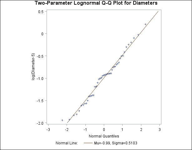
Because the point pattern in Output 5.22.5 is linear, you can estimate the lognormal parameters and as the normal plot estimates of and , which are and . These values correspond to the previous estimates of for and for .