The CORR Procedure

Fisher’s z Transformation

Subsections:

Confidence Limits for the Correlation
Applications of Fisher’s z Transformation

For a sample correlation r that uses a sample from a bivariate normal distribution with correlation $\rho = 0$ , the statistic

$t_ r \, = \, {(n-2)}^{1/2} \, {\left(\frac{r^{2}}{1-r^{2}}\right)}^{1/2}$

has a Student’s t distribution with (n-2) degrees of freedom.

With the monotone transformation of the correlation r (Fisher 1921)

$z_ r \, = \, {\tanh }^{-1} ( r ) \, = \, \frac{1}{2} \, \log \left( \frac{1+r}{1-r} \right)$

the statistic $z_ r$ has an approximate normal distribution with mean and variance

$E(z_ r) \, = \, \zeta \, + \, \frac{\rho }{2(n-1)}$

$V(z_ r) \, = \, \frac{1}{n-3}$

where ${\zeta } = {\tanh }^{-1} ({\rho })$ .

For the transformed $z_ r$ , the approximate variance 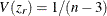$V(z_ r) = 1/(n-3)$ is independent of the correlation $\rho$ . Furthermore, even the distribution of $z_ r$ is not strictly normal, it tends to normality rapidly as the sample size increases for any values of $\rho$ (Fisher 1973, pp. 200–201).

For the null hypothesis $H_0\colon \rho ={\rho }_{0}$ , the p-values are computed by treating

$z_ r - {\zeta }_{0} - \frac{{\rho }_{0}}{2(n-1)}$

as a normal random variable with mean zero and variance $1/(n-3)$ , where ${\zeta }_{0} = {\tanh }^{-1} ({\rho }_{0})$ (Fisher 1973, p. 207; Anderson 1984, p. 123).

Note that the bias adjustment, ${\rho }_{0}/(2(n-1))$ , is always used when computing p-values under the null hypothesis $H_0\colon \rho =\rho _{0}$ in the CORR procedure.

The ALPHA= option in the FISHER option specifies the value $\alpha$ for the confidence level $1-\alpha$ , the RHO0= option specifies the value $\rho _{0}$ in the hypothesis $H_0\colon \rho ={\rho }_{0}$ , and the BIASADJ= option specifies whether the bias adjustment is to be used for the confidence limits.

The TYPE= option specifies the type of confidence limits. The TYPE=TWOSIDED option requests two-sided confidence limits and a p-value under the hypothesis $H_0\colon \rho ={\rho }_{0}$ . For a one-sided confidence limit, the TYPE=LOWER option requests a lower confidence limit and a p-value under the hypothesis $H_0\colon \rho <={\rho }_{0}$ , and the TYPE=UPPER option requests an upper confidence limit and a p-value under the hypothesis $H_0\colon \rho >={\rho }_{0}$ .

Confidence Limits for the Correlation

The confidence limits for the correlation $\rho$ are derived through the confidence limits for the parameter $\zeta$ , with or without the bias adjustment.

Without a bias adjustment, confidence limits for $\zeta$ are computed by treating

$z_ r - \zeta$

as having a normal distribution with mean zero and variance $1/(n-3)$ .

That is, the two-sided confidence limits for $\zeta$ are computed as

${\zeta }_ l = z_ r - z_{(1-\alpha /2)} \, \sqrt {\frac{1}{n-3}}$

${\zeta }_ u = z_ r + z_{(1-\alpha /2)} \, \sqrt {\frac{1}{n-3}}$

where $z_{(1-\alpha /2)}$ is the $100(1-\alpha /2)$ percentage point of the standard normal distribution.

With a bias adjustment, confidence limits for $\zeta$ are computed by treating

$z_ r - \zeta - \mr{bias}(r)$

as having a normal distribution with mean zero and variance $1/(n-3)$ , where the bias adjustment function (Keeping 1962, p. 308) is

$\mr{bias}(r) = \frac{r}{2(n-1)}$

That is, the two-sided confidence limits for $\zeta$ are computed as

${\zeta }_ l = z_ r - \mr{bias}(r) - z_{(1-\alpha /2)} \, \sqrt {\frac{1}{n-3}}$

${\zeta }_ u = z_ r - \mr{bias}(r) + z_{(1-\alpha /2)} \, \sqrt {\frac{1}{n-3}}$

These computed confidence limits of ${\zeta }_ l$ and ${\zeta }_ u$ are then transformed back to derive the confidence limits for the correlation $\rho$ :

$r_{l} = \tanh ( {\zeta }_{l} ) = \frac{ \exp ( 2 {\zeta }_{l}) -1}{ \exp ( 2 {\zeta }_{l}) +1}$

$r_{u} = \tanh ( {\zeta }_{u} ) = \frac{ \exp ( 2 {\zeta }_{u}) -1}{ \exp ( 2 {\zeta }_{u}) +1}$

Note that with a bias adjustment, the CORR procedure also displays the following correlation estimate:

$r_{adj} = \tanh ( z_ r - \mr{bias}(r) )$

Applications of Fisher’s z Transformation

Fisher (1973, p. 199) describes the following practical applications of the z transformation:

testing whether a population correlation is equal to a given value
testing for equality of two population correlations
combining correlation estimates from different samples

To test if a population correlation $\rho _1$ from a sample of $n_1$ observations with sample correlation $r_1$ is equal to a given $\rho _{0}$ , first apply the z transformation to $r_1$ and $\rho _{0}$ : $z_{1} = {\tanh }^{-1} (r_{1})$ and ${\zeta }_{0} = {\tanh }^{-1} ({\rho }_{0})$ .

The p-value is then computed by treating

$z_1 - {\zeta }_{0} - \frac{{\rho }_{0}}{2(n_{1}-1)}$

as a normal random variable with mean zero and variance $1/(n_{1}-3)$ .

Assume that sample correlations $r_{1}$ and $r_{2}$ are computed from two independent samples of $n_1$ and $n_2$ observations, respectively. To test whether the two corresponding population correlations, $\rho _1$ and $\rho _2$ , are equal, first apply the z transformation to the two sample correlations: $z_{1} = {\tanh }^{-1} (r_{1})$ and $z_{2} = {\tanh }^{-1} (r_{2})$ .

The p-value is derived under the null hypothesis of equal correlation. That is, the difference $z_{1} - z_{2}$ is distributed as a normal random variable with mean zero and variance $1/(n_{1}-3) + 1/(n_{2}-3)$ .

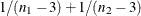Assuming further that the two samples are from populations with identical correlation, a combined correlation estimate can be computed. The weighted average of the corresponding z values is

$\bar{z} = \frac{(n_{1}-3) z_{1} + (n_{2} -3) z_{2}}{n_{1}+n_{2}-6}$

where the weights are inversely proportional to their variances.

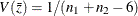Thus, a combined correlation estimate is $\bar{r} = {\tanh } (\bar{z})$ and $V(\bar{z}) = 1 / (n_{1} + n_{2} -6)$ . See Example 2.4 for further illustrations of these applications.

Note that this approach can be extended to include more than two samples.