The UNIVARIATE Procedure
- Overview
-
Getting Started

-
Syntax
-
DetailsMissing ValuesRoundingDescriptive StatisticsCalculating the ModeCalculating PercentilesTests for LocationConfidence Limits for Parameters of the Normal DistributionRobust EstimatorsCreating Line Printer PlotsCreating High-Resolution GraphicsUsing the CLASS Statement to Create Comparative PlotsPositioning InsetsFormulas for Fitted Continuous DistributionsGoodness-of-Fit TestsKernel Density EstimatesConstruction of Quantile-Quantile and Probability PlotsInterpretation of Quantile-Quantile and Probability PlotsDistributions for Probability and Q-Q PlotsEstimating Shape Parameters Using Q-Q PlotsEstimating Location and Scale Parameters Using Q-Q PlotsEstimating Percentiles Using Q-Q PlotsInput Data SetsOUT= Output Data Set in the OUTPUT StatementOUTHISTOGRAM= Output Data SetOUTKERNEL= Output Data SetOUTTABLE= Output Data SetTables for Summary StatisticsODS Table NamesODS Tables for Fitted DistributionsODS GraphicsComputational Resources
-
ExamplesComputing Descriptive Statistics for Multiple VariablesCalculating ModesIdentifying Extreme Observations and Extreme ValuesCreating a Frequency TableCreating Basic Summary PlotsAnalyzing a Data Set With a FREQ VariableSaving Summary Statistics in an OUT= Output Data SetSaving Percentiles in an Output Data SetComputing Confidence Limits for the Mean, Standard Deviation, and VarianceComputing Confidence Limits for Quantiles and PercentilesComputing Robust EstimatesTesting for LocationPerforming a Sign Test Using Paired DataCreating a HistogramCreating a One-Way Comparative HistogramCreating a Two-Way Comparative HistogramAdding Insets with Descriptive StatisticsBinning a HistogramAdding a Normal Curve to a HistogramAdding Fitted Normal Curves to a Comparative HistogramFitting a Beta CurveFitting Lognormal, Weibull, and Gamma CurvesComputing Kernel Density EstimatesFitting a Three-Parameter Lognormal CurveAnnotating a Folded Normal CurveCreating Lognormal Probability PlotsCreating a Histogram to Display Lognormal FitCreating a Normal Quantile PlotAdding a Distribution Reference LineInterpreting a Normal Quantile PlotEstimating Three Parameters from Lognormal Quantile PlotsEstimating Percentiles from Lognormal Quantile PlotsEstimating Parameters from Lognormal Quantile PlotsComparing Weibull Quantile PlotsCreating a Cumulative Distribution PlotCreating a P-P Plot
- References
This example, which is a continuation of Example 4.30, demonstrates techniques for estimating the shape, location, and scale parameters, and the theoretical percentiles for a three-parameter lognormal distribution.
The three-parameter lognormal distribution depends on a threshold parameter ![]() , a scale parameter
, a scale parameter ![]() , and a shape parameter
, and a shape parameter ![]() . You can estimate
. You can estimate ![]() from a series of lognormal Q-Q plots which use the SIGMA= secondary option to specify different values of
from a series of lognormal Q-Q plots which use the SIGMA= secondary option to specify different values of ![]() ; the estimate of
; the estimate of ![]() is the value that linearizes the point pattern. You can then estimate the threshold and scale parameters from the intercept
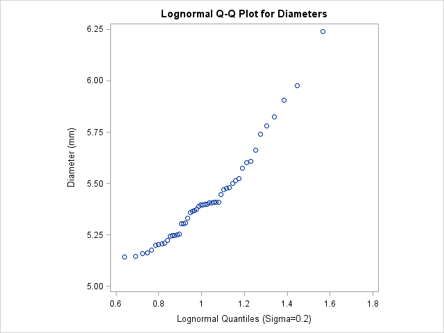
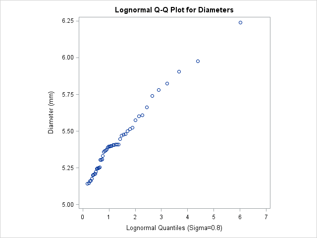
and slope of the point pattern. The following statements create the series of plots in Output 4.31.1, Output 4.31.2, and Output 4.31.3 for
is the value that linearizes the point pattern. You can then estimate the threshold and scale parameters from the intercept
and slope of the point pattern. The following statements create the series of plots in Output 4.31.1, Output 4.31.2, and Output 4.31.3 for ![]() values of 0.2, 0.5, and 0.8, respectively:
values of 0.2, 0.5, and 0.8, respectively:
title 'Lognormal Q-Q Plot for Diameters';
proc univariate data=Measures noprint;
   qqplot Diameter / lognormal(sigma=0.2 0.5 0.8)
                     square
                     odstitle = title;
run;
Note: You must specify a value for the shape parameter ![]() for a lognormal Q-Q plot with the SIGMA= option or its alias, the SHAPE= option.
for a lognormal Q-Q plot with the SIGMA= option or its alias, the SHAPE= option.
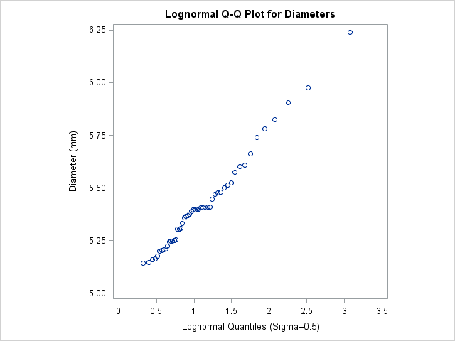
The plot in Output 4.31.2 displays the most linear point pattern, indicating that the lognormal distribution with ![]() provides a reasonable fit for the data distribution.
provides a reasonable fit for the data distribution.
Data with this particular lognormal distribution have the following density function:
The points in the plot fall on or near the line with intercept ![]() and slope
and slope ![]() . Based on Output 4.31.2,
. Based on Output 4.31.2, ![]() and
and ![]() , giving
, giving ![]() .
.
You can also request a reference line by using the SIGMA=, THETA=, and ZETA= options together. The following statements produce the lognormal Q-Q plot in Output 4.31.4:
title 'Lognormal Q-Q Plot for Diameters';
proc univariate data=Measures noprint;
   qqplot Diameter / lognormal(theta=5 zeta=est sigma=est)
                     square
                     odstitle = title;
run;
Output 4.31.1 through Output 4.31.3 show that the threshold parameter ![]() is not equal to zero. Specifying THETA=5 overrides the default value of zero. The SIGMA=EST and ZETA=EST secondary options
request estimates for
is not equal to zero. Specifying THETA=5 overrides the default value of zero. The SIGMA=EST and ZETA=EST secondary options
request estimates for ![]() and
and ![]() that use the sample mean and standard deviation.
that use the sample mean and standard deviation.
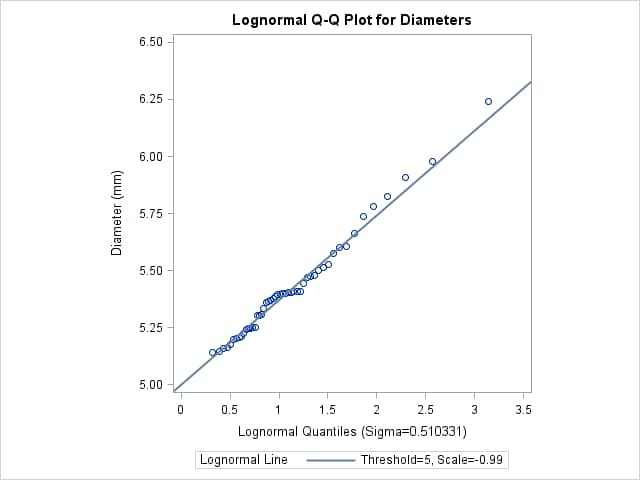
From the plot in Output 4.31.2, ![]() can be estimated as 0.51, which is consistent with the estimate of 0.5 derived from the plot in Output 4.31.2. Example 4.32 illustrates how to estimate percentiles by using lognormal Q-Q plots.
can be estimated as 0.51, which is consistent with the estimate of 0.5 derived from the plot in Output 4.31.2. Example 4.32 illustrates how to estimate percentiles by using lognormal Q-Q plots.
A sample program for this example, uniex18.sas, is available in the SAS Sample Library for Base SAS software.