The Linear Programming Solver
- Overview
- Getting Started
-
Syntax

-
DetailsPresolvePricing Strategies for the Primal and Dual Simplex AlgorithmsThe Network Simplex AlgorithmThe Interior Point AlgorithmIteration Log for the Primal and Dual Simplex AlgorithmsIteration Log for the Network Simplex AlgorithmIteration Log for the Interior Point AlgorithmIteration Log for the Crossover AlgorithmConcurrent LPParallel ProcessingProblem StatisticsVariable and Constraint StatusIrreducible Infeasible SetMacro Variable _OROPTMODEL_
-
ExamplesDiet ProblemReoptimizing the Diet Problem Using BASIS=WARMSTARTTwo-Person Zero-Sum GameFinding an Irreducible Infeasible SetUsing the Network Simplex AlgorithmMigration to OPTMODEL: Generalized NetworksMigration to OPTMODEL: Maximum FlowMigration to OPTMODEL: Production, Inventory, DistributionMigration to OPTMODEL: Shortest Path
- References
Example 7.3 Two-Person Zero-Sum Game
Consider a two-person zero-sum game (where one person wins what the other person loses). The players make moves simultaneously, and each has a choice of actions. There is a payoff matrix that indicates the amount one player gives to the other under each combination of actions:
![\[ \begin{array}{ccc}& & \mr{Player \ II \ plays}\, j \\ & & \begin{array}{rrrr}1 & 2 & 3 & 4 \end{array}\\ \mr{Player \ I \ plays}\, i & \begin{array}{c}1\\ 2\\ 3\end{array}& \left( \begin{array}{rlll} -5 & 3 & 1 & 8\\ 5 & 5 & 4 & 6 \\ -4 & 6 & 0 & 5 \end{array} \right) \end{array} \]](images/ormpug_lpsolver0063.png)
If player I makes move i and player II makes move j, then player I wins (and player II loses)  . What is the best strategy for the two players to adopt? This example is simple enough to be analyzed from observation. Suppose
player I plays 1 or 3; the best response of player II is to play 1. In both cases, player I loses and player II wins. So the
best action for player I is to play 2. In this case, the best response for player II is to play 3, which minimizes the loss.
In this case, (2, 3) is a pure-strategy Nash equilibrium in this game.
. What is the best strategy for the two players to adopt? This example is simple enough to be analyzed from observation. Suppose
player I plays 1 or 3; the best response of player II is to play 1. In both cases, player I loses and player II wins. So the
best action for player I is to play 2. In this case, the best response for player II is to play 3, which minimizes the loss.
In this case, (2, 3) is a pure-strategy Nash equilibrium in this game.
For illustration, consider the following mixed strategy case. Assume that player I selects i with probability  , and player II selects j with probability
  . Consider player II’s problem of minimizing the maximum expected payout:
![\[ \displaystyle \mathop {\min }_{\mathbf{q}}\left\{ \displaystyle \mathop {\max }_{i} \sum _{j = 1}^4 a_{ij}q_ j \right\} \quad {\mathrm{ subject \ to}} \; \; \sum _{j = 1}^4 q_{ij} = 1, \quad \mathbf{q} \geq 0 \]](images/ormpug_lpsolver0067.png)
This is equivalent to
![\[ \begin{array}{rcrccl} \displaystyle \mathop {\min }_{\mathbf{q}, v}\; v & {\mathrm{ subject \ to}} & \displaystyle \mathop \sum _{j = 1}^4 a_{ij}q_ j & \leq & v & \forall \, i \\ & & \displaystyle \mathop \sum _{j=1}^4 q_ j & = & 1 & \\ & & \mathbf{q} & \geq & 0 & \end{array} \]](images/ormpug_lpsolver0068.png)
The problem can be transformed into a more standard format by making a simple change of variables:  . The preceding LP formulation now becomes
![\[ \begin{array}{rcrccl} \displaystyle \mathop {\min }_{\mathbf{x}, v}\; v & {\mathrm{ subject \ to}} & \displaystyle \mathop \sum _{j = 1}^4 a_{ij}x_ j & \leq & 1 & \forall \, i \\ & & \displaystyle \mathop \sum _{j=1}^4 x_ j & = & 1/v & \\ & & \mathbf{q} & \geq & 0 & \end{array} \]](images/ormpug_lpsolver0070.png)
which is equivalent to
![\[ \displaystyle \mathop {\max }_{\mathbf{x}}\; \sum _{j = 1}^4 x_ j \quad {\mathrm{ subject \ to} }\; \; A\mathbf{x} \leq \mathbf{1}, \quad \mathbf{x} \geq 0 \]](images/ormpug_lpsolver0071.png)
where A is the payoff matrix and  is a vector of 1’s. It turns out that the corresponding optimization problem from player I’s perspective can be obtained
by solving the dual problem, which can be written as
is a vector of 1’s. It turns out that the corresponding optimization problem from player I’s perspective can be obtained
by solving the dual problem, which can be written as
![\[ \displaystyle \mathop {\min }_{\mathbf{y}}\; \sum _{i = 1}^3 y_ i \quad {\mathrm{ subject \ to}} \; \; A^\textrm {T}\mathbf{y} \geq \mathbf{1}, \quad \mathbf{y} \geq 0 \]](images/ormpug_lpsolver0073.png)
You can model the problem and solve it by using PROC OPTMODEL as follows:
proc optmodel;
   num a{1..3, 1..4}=[-5 3 1 8
                       5 5 4 6
                      -4 6 0 5];
   var x{1..4} >= 0;
   max f = sum{i in 1..4}x[i];
   con c{i in 1..3}: sum{j in 1..4}a[i,j]*x[j] <= 1;
   solve with lp / algorithm = ps presolver = none logfreq = 1;
   print x;
   print c.dual;
quit;
The optimal solution is displayed in Output 7.3.1.
Output 7.3.1: Optimal Solutions to the Two-Person Zero-Sum Game
| Problem Summary | |
|---|---|
| Objective Sense | Maximization |
| Objective Function | f |
| Objective Type | Linear |
| Number of Variables | 4 |
| Bounded Above | 0 |
| Bounded Below | 4 |
| Bounded Below and Above | 0 |
| Free | 0 |
| Fixed | 0 |
| Number of Constraints | 3 |
| Linear LE (<=) | 3 |
| Linear EQ (=) | 0 |
| Linear GE (>=) | 0 |
| Linear Range | 0 |
| Constraint Coefficients | 11 |
The optimal solution 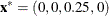 with an optimal value of 0.25. Therefore the optimal strategy for player II is
 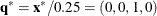 . You can check the optimal solution of the dual problem by using the constraint suffix ".dual". So
  and player I’s optimal strategy is (0, 1, 0). The solution is consistent with our intuition from observation.