The OPTLP Procedure
- Overview
- Getting Started
-
Syntax

-
Details
Data Input and Output Presolve Pricing Strategies for the Primal and Dual Simplex Solvers Warm Start for the Primal and Dual Simplex Solvers The Network Simplex Algorithm The Interior Point Algorithm Iteration Log for the Primal and Dual Simplex Solvers Iteration Log for the Network Simplex Solver Iteration Log for the Interior Point Solver ODS Tables Irreducible Infeasible Set Memory Limit PROC OPTLP Macro Variable
-
Examples
- References
Example 10.8 Using the Network Simplex Solver
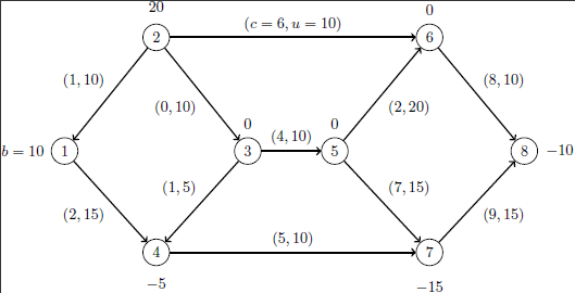
This example demonstrates how to use the network simplex solver to find the minimum-cost flow in a directed graph. Consider the directed graph in Figure 10.5, which appears in Ahuja, Magnanti, and Orlin (1993).
Figure 10.5
Minimum Cost Network Flow Problem: Data
You can use the following SAS statements to create the input data set ex8:
data ex8;
   input field1 $8. field2 $13. @25 field3 $13. field4  @53 field5 $13. field6;
   datalines;
NAME    .               .                    .      .                   .
ROWS    .               .                    .      .                   .
N       obj             .                    .      .                   .
E       balance['1']    .                    .      .                   .
E       balance['2']    .                    .      .                   .
E       balance['3']    .                    .      .                   .
E       balance['4']    .                    .      .                   .
E       balance['5']    .                    .      .                   .
E       balance['6']    .                    .      .                   .
E       balance['7']    .                    .      .                   .
E       balance['8']    .                    .      .                   .
COLUMNS .               .                    .      .                   .
.       x['1','4']      obj                  2      balance['1']        1
.       x['1','4']      balance['4']        -1      .                   .
.       x['2','1']      obj                  1      balance['1']       -1
.       x['2','1']      balance['2']         1      .                   .
.       x['2','3']      balance['2']         1      balance['3']       -1
.       x['2','6']      obj                  6      balance['2']        1
.       x['2','6']      balance['6']        -1      .                   .
.       x['3','4']      obj                  1      balance['3']        1
.       x['3','4']      balance['4']        -1      .                   .
.       x['3','5']      obj                  4      balance['3']        1
.       x['3','5']      balance['5']        -1      .                   .
.       x['4','7']      obj                  5      balance['4']        1
.       x['4','7']      balance['7']        -1      .                   .
.       x['5','6']      obj                  2      balance['5']        1
.       x['5','6']      balance['6']        -1      .                   .
.       x['5','7']      obj                  7      balance['5']        1
.       x['5','7']      balance['7']        -1      .                   .
.       x['6','8']      obj                  8      balance['6']        1
.       x['6','8']      balance['8']        -1      .                   .
.       x['7','8']      obj                  9      balance['7']        1
.       x['7','8']      balance['8']        -1      .                   .
RHS     .               .                    .      .                   .
.       .RHS.           balance['1']        10      .                   .
.       .RHS.           balance['2']        20      .                   .
.       .RHS.           balance['4']        -5      .                   .
.       .RHS.           balance['7']       -15      .                   .
.       .RHS.           balance['8']       -10      .                   .
BOUNDS  .               .                    .      .                   .
UP      .BOUNDS.        x['1','4']          15      .                   .
UP      .BOUNDS.        x['2','1']          10      .                   .
UP      .BOUNDS.        x['2','3']          10      .                   .
UP      .BOUNDS.        x['2','6']          10      .                   .
UP      .BOUNDS.        x['3','4']           5      .                   .
UP      .BOUNDS.        x['3','5']          10      .                   .
UP      .BOUNDS.        x['4','7']          10      .                   .
UP      .BOUNDS.        x['5','6']          20      .                   .
UP      .BOUNDS.        x['5','7']          15      .                   .
UP      .BOUNDS.        x['6','8']          10      .                   .
UP      .BOUNDS.        x['7','8']          15      .                   .
ENDATA  .               .                    .      .                   .
;
You can use the following call to PROC OPTLP to find the minimum-cost flow:
proc optlp
  presolver  = none
  printlevel = 2
  printfreq  = 1
  data       = ex8
  primalout  = ex8out
  solver     = ns;
run;
The optimal solution is displayed in Output 10.8.1.
Output 10.8.1
Network Simplex Solver: Primal Solution Output
| The OPTLP Procedure |
| Primal Solution |
| Obs | Objective Function ID |
RHS ID | Variable Name | Variable Type |
Objective Coefficient |
Lower Bound |
Upper Bound | Variable Value |
Variable Status |
Reduced Cost |
|---|---|---|---|---|---|---|---|---|---|---|
| 1 | obj | .RHS. | x['1','4'] | D | 2 | 0 | 15 | 10 | B | 0 |
| 2 | obj | .RHS. | x['2','1'] | D | 1 | 0 | 10 | 0 | L | 1 |
| 3 | obj | .RHS. | x['2','3'] | D | 0 | 0 | 10 | 10 | B | 0 |
| 4 | obj | .RHS. | x['2','6'] | D | 6 | 0 | 10 | 10 | B | 0 |
| 5 | obj | .RHS. | x['3','4'] | D | 1 | 0 | 5 | 5 | U | -1 |
| 6 | obj | .RHS. | x['3','5'] | D | 4 | 0 | 10 | 5 | B | 0 |
| 7 | obj | .RHS. | x['4','7'] | D | 5 | 0 | 10 | 10 | B | -4 |
| 8 | obj | .RHS. | x['5','6'] | D | 2 | 0 | 20 | 0 | L | 0 |
| 9 | obj | .RHS. | x['5','7'] | D | 7 | 0 | 15 | 5 | B | 0 |
| 10 | obj | .RHS. | x['6','8'] | D | 8 | 0 | 10 | 10 | B | 0 |
| 11 | obj | .RHS. | x['7','8'] | D | 9 | 0 | 15 | 0 | L | 6 |
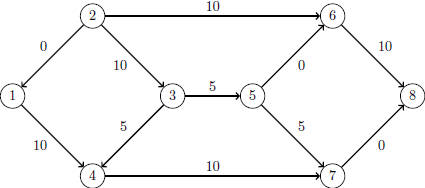
The optimal solution is represented graphically in Figure 10.6.
Figure 10.6
Minimum Cost Network Flow Problem: Optimal Solution
The iteration log is displayed in Output 10.8.2.
Output 10.8.2
Log: Solution Progress
| The OPTLP Procedure |
| NOTE: The problem has 11 variables (0 free, 0 fixed). |
| NOTE: The problem has 8 constraints (0 LE, 8 EQ, 0 GE, 0 range). |
| NOTE: The problem has 22 constraint coefficients. |
| NOTE: The OPTLP presolver value NONE is applied. |
| NOTE: The NETWORK SIMPLEX solver is called. |
| NOTE: The network has 8 rows (100.00%), 11 columns (100.00%), and 1 component. |
| NOTE: The network extraction and setup time is 0.00 seconds. |
| Iteration PrimalObj PrimalInf Time |
| 1 0 20.0000000 0.00 |
| 2 0 20.0000000 0.00 |
| 3 5.0000000 15.0000000 0.00 |
| 4 5.0000000 15.0000000 0.00 |
| 5 75.0000000 15.0000000 0.00 |
| 6 75.0000000 15.0000000 0.00 |
| 7 130.0000000 10.0000000 0.00 |
| 8 270.0000000 0 0.00 |
| NOTE: The Network Simplex solve time is 0.00 seconds. |
| NOTE: The total Network Simplex solve time is 0.00 seconds. |
| NOTE: Optimal. |
| NOTE: Objective = 270. |
| NOTE: The data set WORK.EX8OUT has 11 observations and 10 variables. |