The OPTLP Procedure

Overview: OPTLP Procedure

The OPTLP procedure provides four methods of solving linear programs (LPs). A linear program has the following formulation:

$\text{[math]}$

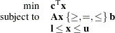where

$\text{[math]}$	$\text{[math]}$	$\text{[math]}$	is the vector of decision variables
$\text{[math]}$	$\text{[math]}$	$\text{[math]}$	is the matrix of constraints
$\text{[math]}$	$\text{[math]}$	$\text{[math]}$	is the vector of objective function coefficients
$\text{[math]}$	$\text{[math]}$	$\text{[math]}$	is the vector of constraints right-hand sides (RHS)
$\text{[math]}$	$\text{[math]}$	$\text{[math]}$	is the vector of lower bounds on variables
$\text{[math]}$	$\text{[math]}$	$\text{[math]}$	is the vector of upper bounds on variables

The following LP solvers are available in the OPTLP procedure:

primal simplex solver
dual simplex solver
network simplex solver
interior point solver

The primal and dual simplex solvers implement the two-phase simplex method. In phase I, the solver tries to find a feasible solution. If no feasible solution is found, the LP is infeasible; otherwise, the solver enters phase II to solve the original LP. The network simplex solver extracts a network substructure, solves this using network simplex, and then constructs an advanced basis to feed to either primal or dual simplex. The interior point solver implements a primal-dual predictor-corrector interior point algorithm.

PROC OPTLP requires a linear program to be specified using a SAS data set that adheres to the MPS format, a widely accepted format in the optimization community. For details about the MPS format see Chapter 9, The MPS-Format SAS Data Set.

You can use the MPSOUT= option to convert typical PROC LP format data sets into MPS-format SAS data sets. The option is available in the LP, INTPOINT, and NETFLOW procedures. For details about this option, see Chapter 5, The LP Procedure (SAS/OR User's Guide: Mathematical Programming Legacy Procedures), Chapter 4, The INTPOINT Procedure (SAS/OR User's Guide: Mathematical Programming Legacy Procedures), and Chapter 6, The NETFLOW Procedure (SAS/OR User's Guide: Mathematical Programming Legacy Procedures).