The Linear Programming Solver

Getting Started: LP Solver

The following example illustrates how you can use the OPTMODEL procedure to solve linear programs. Suppose you want to solve the following problem:

$\text{[math]}$

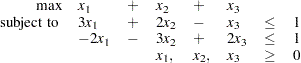You can use the following statements to call the OPTMODEL procedure for solving linear programs:

proc optmodel;
   var x{i in 1..3} >= 0;
   max f =    x[1] +   x[2] +   x[3];
   con c1:  3*x[1] + 2*x[2] -   x[3] <= 1;
   con c2: -2*x[1] - 3*x[2] + 2*x[3] <= 1;
   solve with lp / solver = ps presolver = none printfreq = 1;
   print x;
quit;

The optimal solution and the optimal objective value are displayed in Figure 5.1.

Figure 5.1 Solution Summary

The OPTMODEL Procedure

Problem Summary
Objective Sense	Maximization
Objective Function	f
Objective Type	Linear

Number of Variables	3
Bounded Above	0
Bounded Below	3
Bounded Below and Above	0
Free	0
Fixed	0

Number of Constraints	2
Linear LE (<=)	2
Linear EQ (=)	0
Linear GE (>=)	0
Linear Range	0

Constraint Coefficients	6

Solution Summary
Solver	Primal Simplex
Objective Function	f
Solution Status	Optimal
Objective Value	8
Iterations	2

Primal Infeasibility	0
Dual Infeasibility	0
Bound Infeasibility	0

[1]	x
1	0
2	3
3	5

The iteration log displaying problem statistics, progress of the solution, and the optimal objective value is shown in Figure 5.2.

Figure 5.2 Log

NOTE: The problem has 3 variables (0 free, 0 fixed).

NOTE: The problem has 2 linear constraints (2 LE, 0 EQ, 0 GE, 0 range).

NOTE: The problem has 6 linear constraint coefficients.

NOTE: The problem has 0 nonlinear constraints (0 LE, 0 EQ, 0 GE, 0 range).

NOTE: The OPTLP presolver value NONE is applied.

NOTE: The PRIMAL SIMPLEX solver is called.

Objective Entering Leaving

Phase Iteration Value Variable Variable

2 1 0.500000 x[3] c2 (S)

2 2 8.000000 x[2] c1 (S)

NOTE: Optimal.

NOTE: Objective = 8.