Previous Page

|

Next Page

Example 13.3: Choosing a Good Starting Point

To solve a constrained nonlinear optimization problem, both the optimal primal and optimal dual variables have to be computed. Therefore, a good estimate of both the primal and dual variables is essential for fast convergence. An important feature of the SQP solver is that it computes a good estimate of the dual variables if an estimate of the primal variables is known.

The following example illustrates how a good initial starting point helps in securing the desired optimum:

Assume the starting point = (30, - 30). The SAS code is as follows:

    proc optmodel;
       var x {1..2} <= 8 >= -10;   /* variable bounds */
           
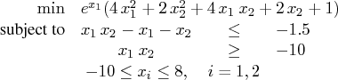
       minimize obj = 
          exp(x[1])*(4*x[1]^2 + 2*x[2]^2 + 4*x[1]*x[2] + 2*x[2] + 1);
       
       con consl: 
          x[1]*x[2] -x[1] - x[2] <= -1.5;
       con cons2:
          x[1]*x[2] >= -10;
       
       x[1] = 30; x[2] = -30; /* starting point */
       solve with sqp / printfreq = 5 ;
       print x;
 

The solution (a local optimum) obtained by the SQP solver is displayed in Output 13.3.1.

You can find a solution with a smaller objective value by assuming a starting point of ( - 10, 1). Continue to submit the following code:

       
       /* starting point */
       x[1] = -10;
       x[2] =  1;
       
       solve with sqp / printfreq = 5 ;
       print x;
       quit;
 

The corresponding solution is displayed in Output 13.3.2.

The preceding illustration demonstrates the importance of a good starting point in obtaining the optimal solution. The SQP solver ensures global convergence only to a local optimum. Therefore you need to have sufficient knowledge of your problem in order to be able to get a "good" estimate of the starting point.