The NLPC Nonlinear Optimization Solver

Example 10.1: Least-Squares Problem

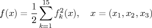
Although the current release of the NLPC solver does not implement techniques specialized for least-squares problems, this example illustrates how the NLPC solver can solve least-squares problems by using general nonlinear optimization techniques. The following Bard function (see Moré, Garbow, and Hillstrom 1981) is a least-squares problem with 3 parameters and 15 residual functions :

where

with , , , and

The minimum function value E - 3 is at the point . The starting point is used.

You can use the following SAS code to formulate and solve this least-squares problem:

    proc optmodel;
       set S = 1..15;
       number u{k in S} = k;
       number v{k in S} = 16 - k;
       number w{k in S} = min(u[k], v[k]);
       number y{S} = [ .14 .18 .22 .25 .29 .32 .35 .39 .37 .58
                       .73 .96 1.34 2.10 4.39 ];
       var x{1..3} init 1;
       
       min f = 0.5*sum{k in S} ( y[k] -
                 ( x[1] + u[k]/(v[k]*x[2] + w[k]*x[3]) )
               )^2;
 
       solve with nlpc / printfreq=1;
       print x;
    quit;
 

A problem summary is displayed in Figure 10.1.1. Since there is no explicit optimization technique specified (using the TECH= option), the default algorithm of the trust region method is used. Figure 10.1.2 displays the iteration log. The solution summary and the solution are shown in Figure 10.1.3.

Output 10.1.1: Least-Squares Problem Solved with TRUREG: Problem Summary

Problem Summary Objective Sense Minimization Objective Function f Objective Type Nonlinear     Number of Variables 3 Bounded Above 0 Bounded Below 0 Bounded Below and Above 0 Free 3 Fixed 0     Number of Constraints 0

Output 10.1.2: Least-Squares Problem Solved with TRUREG: Iteration Log

Iteration Log: Trust Region Method Iter Function Calls Objective Value Optimality Error Trust Region Radius 0 0 20.8408 1.2445 . 1 1 2.8333 2.7031 1.000 2 2 0.6302 2.3180 0.989 3 3 0.1077 0.7732 0.998 4 4 0.009011 0.1396 1.007 5 5 0.004134 0.0125 1.042 6 6 0.004107 0.0000805 0.199 7 7 0.004107 4.3523E-8 0.0207 Note: Optimality criteria (ABSOPTTOL=0.001, RELOPTTOL=1E-6) are satisfied.

Output 10.1.3: Least-Squares Problem Solved with TRUREG: Solution

Solution Summary Solver NLPC/Trust Region Objective Function f Solution Status Optimal Objective Value 0.0041074387 Iterations 7     Absolute Optimality Error 4.352335E-8 Relative Optimality Error 4.352335E-8 Absolute Infeasibility 0 Relative Infeasibility 0 [1] x 1 0.082411 2 1.133036 3 2.343696

Alternatively, you can specify the Newton-type method with line search by using the following statement:

       solve with nlpc / tech=newtyp printfreq=1;
 

You get the output for the NEWTYP method as shown in Figure 10.1.4 and Figure 10.1.5.

Output 10.1.4: Least-Squares Problem Solved with NEWTYP: Iteration Log

Iteration Log: Newton-Type Method with Line Search Iter Function Calls Objective Value Optimality Error Step Size Slope of Search Direction 0 0 20.8408 1.2445 . . 1 1 2.2590 2.6880 1.000 -35.485 2 2 0.6235 2.3158 1.000 -2.577 3 3 0.1116 0.7488 1.000 -0.831 4 4 0.0115 0.1703 1.000 -0.172 5 5 0.004188 0.0167 1.000 -0.0136 6 6 0.004109 0.000427 1.000 -0.0002 7 7 0.004109 0.0000637 1.000 -578E-9 8 8 0.004108 0.0000352 1.000 -95E-8 9 9 0.004107 8.7568E-6 1.000 -52E-8 10 10 0.004107 1.1411E-6 1.000 -33E-9 11 11 0.004107 8.2006E-8 1.000 -63E-11 Note: Optimality criteria (ABSOPTTOL=0.001, RELOPTTOL=1E-6) are satisfied.

Output 10.1.5: Least-Squares Problem Solved with NEWTYP: Solution

Solution Summary Solver NLPC/Newton-Type Objective Function f Solution Status Optimal Objective Value 0.0041074387 Iterations 11     Absolute Optimality Error 8.2005644E-8 Relative Optimality Error 8.2005644E-8 Absolute Infeasibility 0 Relative Infeasibility 0 [1] x 1 0.082411 2 1.133059 3 2.343674

You can also select the conjugate gradient method as follows:

       solve with nlpc / tech=congra printfreq=2;
 

Note that the PRINTFREQ= option was used to reduce the number of rows in the iteration log. As Figure 10.1.6 shows, only every other iteration is displayed. Figure 10.1.7 gives a summary of the solution and prints the solution.

Output 10.1.6: Least-Squares Problem Solved with CONGRA: Iteration Log

Iteration Log: Conjugate Gradient Method Iter Function Calls Objective Value Optimality Error Step Size Slope of Search Direction Restarts 0 0 20.8408 1.2445 . . 0 2 4 0.7199 1.1503 0.108 -11.045 1 4 10 0.0119 0.4362 0.150 -0.0010 2 6 14 0.004903 0.008169 35.849 -0.0001 3 8 19 0.004788 0.0819 22.628 -0.0001 4 10 24 0.004233 0.0436 0.679 -0.0034 6 12 28 0.004201 0.0191 0.345 -0.0001 7 14 32 0.004166 0.0161 20.000 -129E-7 8 16 36 0.004160 0.003508 0.112 -205E-8 9 18 40 0.004108 0.001920 9.125 -108E-7 10 20 44 0.004108 0.000637 2.000 -178E-9 12 22 48 0.004107 0.000581 0.291 -245E-9 13 24 52 0.004107 2.5337E-6 2.000 -62E-13 14 25 54 0.004107 7.4262E-8 0.142 -15E-12 14 Note: Optimality criteria (ABSOPTTOL=0.001, RELOPTTOL=1E-6) are satisfied.

Output 10.1.7: Least-Squares Problem Solved with CONGRA: Solution

Solution Summary Solver NLPC/Conjugate Gradient Objective Function f Solution Status Optimal Objective Value 0.0041074387 Iterations 25     Absolute Optimality Error 7.4261706E-8 Relative Optimality Error 7.4261706E-8 Absolute Infeasibility 0 Relative Infeasibility 0 [1] x 1 0.082411 2 1.133038 3 2.343693

Although the number of iterations required for each optimization technique to converge varies, all three techniques produce the identical solution, given the same starting point.