IMSTAT Procedure (Analytics)

Example 13: Forecasting with Goal Seeking

Details

This IMSTAT procedure example demonstrates using FORECAST statement with a goal-seeking analysis.

Goal seeking is based on numerical optimization of control variables in order to produce a desired forecast. You can think of it as an inverse prediction method. Normal prediction techniques produce a predicted value when given a series of inputs. An inverse prediction method specifies the desired predicted value and then asks to find the inputs that generate it. For time series forecasting, the inverse prediction method is called goal seeking. Instead of producing a forecast for values of independent variables that you provide, you provide the target forecast (the goal). Then, the numerical optimization attempts to find the values of the independent variables that generate the goal values for the chosen model.

The independent variables in the time series model are divided into two categories. Those whose values can be modified during goal seeking are called controllable variables. The values of other independent variables are immutable during goal seeking. You specify the variables that can be modified during goal seeking in the CONTROL= option. You specify the variable that cannot be modified (the target) with the GOAL= option.

Program

data work.pricedata;   1
    set sashelp.pricedata; 
    where region=1 and product=1 and line=1;
run;

data work.goalsale;
    retain slast 0;
    keep region product line;
    keep date gsale;
    set pricedata end=last;
    if sale ne . then slast=sale;
    if last then do;
        gsale=slast;
        do i=1 to 4;  2
            gsale=1.05 * gsale;
            date=intnx("month", date, 1);
            output;
        end;
        stop;
    end;
run;

data work.merged;
    merge pricedata goalsale;
    by date;
run;

/*
proc print data=merged;  3
    var date sale price discount gsale;
    where date > '01jul2002'd;
run;
*/

proc imstat;
     forecast data=merged date / dep    =sale  4
                                 control=(price discount)
                                 goal   =gsale
                                 info
                                 lead   =4
                                 host   ="grid001.example.com"  5
                                 port   =10010;
quit;

Program Description

The DATA step places a subset of the Sashelp.Pricedata data set into the temporary Work library.
The purpose of this DATA step is to generate four additional observations for the variable Gsale. The values for this variable represent the sales goal to attain.
The PRINT procedure can be used to view the last few observations from the original data set with the observed values for Sale and the target values for variable Gsale.
The FORECAST statement requests a goal seeking analysis for time stamp Date, with dependent variable Sale, control variables Price and Discount, and the goal variable Gsale.
This example also demonstrates how the DATA= option can be used with the HOST= and PORT= option to analyze a data set that is not in memory. This feature is unique to this statement. In this example, the Merged data set is transferred from the temporary Work library to the server and then analyzed.

Output

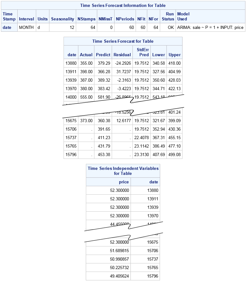
The forecast information table shows that the automatic modeling step determined that the best-fitting model was an ARIMA model with independent variable Price.

Based on this model, the missing values for the control variables are replaced with forecasted values and the result is passed to the goal-seeking analysis. It produces the second and third tables.

The first sixty observations in the forecast table are the forecasted values from the automatic modeling step. The four observations at the end of the table are the result of goal seeking. Notice that the values in the Predict column for these four observations match the values for the Gsale column in the Merged data set. (The data set is not shown here, but is available if you remove the comments from the PROC PRINT statement.) The numerical optimization converged and the goal was met.

The third table, the independent variables table, shows the value for the control variable (Price). The first sixty values for Price match the values in the input table. The last four values for the Price variable are the values for the control variable that produces the goal forecast.