| Nonlinear Optimization Examples |
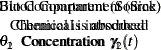
Example 14.3 Compartmental Analysis
Numerical Considerations
An important class of nonlinear models involves a dynamic description of the response rather than an explicit description. These models arise often in chemical kinetics, pharmacokinetics, and ecological compartmental modeling. Two examples are presented in this section. Refer to Bates and Watts (1988) for a more general introduction to the topic.
In this class of problems, function evaluations, as well as gradient evaluations, are not done in full precision. Evaluating a function involves the numerical solution of a differential equation with some prescribed precision. Therefore, two choices exist for evaluating first- and second-order derivatives:
differential equation approach
finite-difference approach
In the differential equation approach, the components of the Hessian and the gradient are written as a solution of a system of differential equations that can be solved simultaneously with the original system. However, the size of a system of differential equations,  , would suddenly increase to
  . This huge increase makes the finite difference approach an easier one.
With the finite-difference approach, a very delicate balance of all the precision requirements of every routine must exist. In the examples that follow, notice the relative levels of precision that are imposed on different modules. Since finite differences are used to compute the first- and second-order derivatives, it is incorrect to set the precision of the ODE solver at a coarse level because that would render the numerical estimation of the finite differences worthless.
A coarse computation of the solution of the differential equation cannot be accompanied by very fine computation of the finite-difference estimates of the gradient and the Hessian. That is, you cannot set the precision of the differential equation solver to be 1E 4 and perform the finite difference estimation with a precision of 1E10.
In addition, this precision must be well-balanced with the termination criteria imposed on the optimization process.
In general, if the precision of the function evaluation is  , the gradient should be computed by finite differences
  , and the Hessian should be computed with finite differences
  . 1
. 1
Diffusion of Tetracycline
Consider the concentration of tetracycline hydrochloride in blood serum. The tetracycline is administered to a subject orally, and the concentration of the tetracycline in the serum is measured. The biological system to be modeled consists of two compartments: a gut compartment in which tetracycline is injected and a blood compartment that absorbs the tetracycline from the gut compartment for delivery to the body. Let  and
and  be the concentrations at time
  in the gut and the serum, respectively. Let
  and
and  be the transfer parameters. The model is depicted as follows.
The rates of flow of the drug are described by the following pair of ordinary differential equations:
 |
 |
 |
|||
 |
|
 |
The initial concentration of the tetracycline in the gut is unknown, and while the concentration in the blood can be measured at all times, initially it is assumed to be zero. Therefore, for the differential equation, the initial conditions are given by
 |
|
 |
|||
 |
|
 |
Also, a nonnegativity constraint is imposed on the parameters , , and  , although for numerical purposes, you might need to use a small value instead of zero for these bounds (such as 1E7).
Suppose  is the observed serum concentration at time
  . The parameters are estimated by minimizing the sum of squares of the differences between the observed and predicted serum concentrations:
 |
The following IML program illustrates how to combine the NLPDD subroutine and the ODE subroutine to estimate the parameters  of this model. The input data are the measurement time and the concentration of the tetracycline in the blood. For more information about the ODE call, see the section ODE Call.
   data tetra;
      input t c @@;
      datalines;
    1 0.7   2 1.2   3 1.4   4 1.4   6 1.1
    8 0.8  10 0.6  12 0.5  16 0.3
   ;

   proc iml;
      use tetra;
      read all into tetra;
      start f(theta) global(thmtrx,t,h,tetra,eps);
         thmtrx = ( -theta[1] || 0 )     //
                  (  theta[1] || -theta[2] );
         c = theta[3]//0 ;
         t = 0 // tetra[,1];
         call ode( r1, "der",c , t, h) j="jac" eps=eps;
         f = ssq((r1[2,])`-tetra[,2]);
         return(f);
      finish;

      start der(t,x) global(thmtrx);
         y = thmtrx*x;
         return(y);
      finish;

      start jac(t,x) global(thmtrx);
         y = thmtrx;
         return(y);
      finish;

      h      = {1.e-14 1. 1.e-5};
      opt    = {0 2 0 1 };
      tc     = repeat(.,1,12);
      tc[1]  = 100;
      tc[7]  = 1.e-8;
      par    = { 1.e-13 . 1.e-10 . . . . };
      con    = j(1,3,0.);
      itheta = { .1  .3  10};
      eps    = 1.e-11;

      call nlpdd(rc,rx,"f",itheta) blc=con opt=opt tc=tc par=par;
The output from the optimization process is shown in Output 14.3.1.
| Parameter Estimates | 3 |
|---|---|
| Lower Bounds | 3 |
| Upper Bounds | 0 |
| Optimization Start | |||
|---|---|---|---|
| Active Constraints | 0 | Objective Function | 4.1469872322 |
| Max Abs Gradient Element | 76.532450643 | Radius | 1 |
| Iteration | Restarts | Function Calls |
Active Constraints |
Objective Function |
Objective Function Change |
Max Abs Gradient Element |
Lambda | Slope of Search Direction |
||
|---|---|---|---|---|---|---|---|---|---|---|
| 1 | 0 | 5 | 0 | 3.12253 | 1.0245 | 124.4 | 67.118 | -8.018 | ||
| 2 | 0 | 6 | 0 | 0.89532 | 2.2272 | 14.1416 | 1.885 | -5.021 | ||
| 3 | 0 | 7 | 0 | 0.32357 | 0.5718 | 3.6959 | 1.186 | -0.785 | ||
| 4 | 0 | 8 | 0 | 0.14689 | 0.1767 | 2.6865 | 0 | -0.122 | ||
| 5 | 0 | 9 | 0 | 0.07485 | 0.0720 | 2.3242 | 0 | -0.0570 | ||
| 6 | 0 | 10 | 0 | 0.06552 | 0.00934 | 1.5950 | 0 | -0.0077 | ||
| 7 | 0 | 11 | 0 | 0.06419 | 0.00133 | 1.1065 | 0 | -0.0010 | ||
| 8 | 0 | 12 | 0 | 0.06334 | 0.000851 | 0.5580 | 0 | -0.0006 | ||
| 9 | 0 | 13 | 0 | 0.06286 | 0.000475 | 0.0815 | 0.0978 | -0.0004 | ||
| 10 | 0 | 14 | 0 | 0.06278 | 0.000084 | 0.0197 | 0.149 | -0.0001 | ||
| 11 | 0 | 15 | 0 | 0.06276 | 0.000019 | 0.0208 | 0 | -135E-7 | ||
| 12 | 0 | 16 | 0 | 0.06274 | 0.000015 | 0.0197 | 0.378 | -103E-7 | ||
| 13 | 0 | 17 | 0 | 0.06270 | 0.000044 | 0.0258 | 0.786 | -506E-7 | ||
| 14 | 0 | 18 | 0 | 0.06265 | 0.000047 | 0.0383 | 0.717 | -402E-7 | ||
| 15 | 0 | 19 | 0 | 0.06242 | 0.000233 | 0.0548 | 0.109 | -0.0001 | ||
| 16 | 0 | 21 | 0 | 0.06038 | 0.00204 | 0.2604 | 0 | -0.0015 | ||
| 17 | 0 | 22 | 0 | 0.05834 | 0.00204 | 0.4049 | 0.0683 | -0.0012 | ||
| 18 | 0 | 23 | 0 | 0.05220 | 0.00614 | 1.3039 | 0.246 | -0.0057 | ||
| 19 | 0 | 24 | 0 | 0.04828 | 0.00392 | 2.0190 | 0 | -0.0041 | ||
| 20 | 0 | 25 | 0 | 0.04085 | 0.00743 | 0.8804 | 0 | -0.0058 | ||
| 21 | 0 | 26 | 0 | 0.03941 | 0.00144 | 0.2781 | 1.795 | -0.0012 | ||
| 22 | 0 | 29 | 0 | 0.03789 | 0.00152 | 0.2194 | 0.570 | -0.0015 | ||
| 23 | 0 | 30 | 0 | 0.03677 | 0.00112 | 0.2226 | 0.547 | -0.0010 | ||
| 24 | 0 | 31 | 0 | 0.03588 | 0.000888 | 0.2334 | 0 | -0.0008 | ||
| 25 | 0 | 32 | 0 | 0.03574 | 0.000145 | 0.0476 | 0 | -0.0002 | ||
| 26 | 0 | 34 | 0 | 0.03566 | 0.000080 | 0.0279 | 0.228 | -0.0001 | ||
| 27 | 0 | 35 | 0 | 0.03565 | 4.457E-6 | 0.0316 | 0 | -249E-7 | ||
| 28 | 0 | 36 | 0 | 0.03565 | 3.579E-6 | 0.00258 | 0 | -263E-8 | ||
| 29 | 0 | 37 | 0 | 0.03565 | 5.199E-7 | 0.00640 | 1.915 | -145E-8 | ||
| 30 | 0 | 38 | 0 | 0.03565 | 3.393E-7 | 0.000816 | 0 | -187E-9 | ||
| 31 | 0 | 39 | 0 | 0.03565 | 1.868E-7 | 0.0143 | 0.452 | -529E-9 | ||
| 32 | 0 | 41 | 0 | 0.03565 | 1.848E-7 | 0.0155 | 1.362 | -368E-9 | ||
| 33 | 0 | 42 | 0 | 0.03565 | 6.235E-7 | 0.000794 | 0 | -733E-9 | ||
| 34 | 0 | 47 | 0 | 0.03565 | 4.44E-10 | 0.000932 | 3.986 | -43E-10 | ||
| 35 | 0 | 48 | 0 | 0.03565 | 4.149E-9 | 0.00117 | 2.000 | -45E-10 | ||
| 36 | 0 | 51 | 0 | 0.03565 | 1.88E-12 | 0.00205 | 101.7 | -38E-10 |
| Optimization Results | |||
|---|---|---|---|
| Iterations | 36 | Function Calls | 52 |
| Gradient Calls | 38 | Active Constraints | 0 |
| Objective Function | 0.0356491964 | Max Abs Gradient Element | 0.0020521614 |
| Slope of Search Direction | -3.762779E-9 | Radius | 1 |
The differential equation model is linear, and in fact, it can be solved by using an eigenvalue decomposition (this is not always feasible without complex arithmetic). Alternately, the availability and the simplicity of the closed form representation of the solution enable you to replace the solution produced by the ODE routine with the simpler and faster analytical solution. Closed forms are not expected to be easily available for nonlinear systems of differential equations, which is why the preceding solution was introduced.
The closed form of the solution requires a change to the function  . The functions needed as arguments of the ODE routine, namely the der and jac modules, can be removed. Here is the revised code:
   start f(th) global(theta,tetra);
      theta = th;
      vv    = v(tetra[,1]);
      error = ssq(vv-tetra[,2]);
      return(error);
   finish;

   start v(t) global(theta);
      v = theta[3]*theta[1]/(theta[2]-theta[1])*
              (exp(-theta[1]*t)-exp(-theta[2]*t));
      return(v);
   finish;

   call nlpdd(rc,rx,"f",itheta) blc=con opt=opt tc=tc par=par;
The parameter estimates, which are shown in Output 14.3.2, are close to those obtained by the first solution.
Because of the nature of the closed form of the solution, you might want to add an additional constraint to guarantee that  at any time during the optimization. This prevents a possible division by
  or a value near in the execution of the
  function. For example, you might add the constraint
 |
Chemical Kinetics of Pyrolysis of Oil Shale
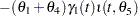
Pyrolysis is a chemical change effected by the action of heat, and this example considers the pyrolysis of oil shale described in Ziegel and Gorman (1980). Oil shale contains organic material that is bonded to the rock. To extract oil from the rock, heat is applied, and the organic material is decomposed into oil, bitumen, and other byproducts. The model is given by
|
|
 |
|||
|
|
 |
|||
 |
|
 |
with the initial conditions
 |
A dead time is assumed to exist in the process. That is, no change occurs up to time  . This is controlled by the indicator function
  , which is given by
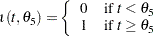 |
where  . Only one of the cases in Ziegel and Gorman (1980) is analyzed in this report, but the others can be handled in a similar manner. The following IML program illustrates how to combine the NLPQN subroutine and the ODE subroutine to estimate the parameters
  in this model:
   data oil ( drop=temp);
      input temp time bitumen oil;
      datalines;
   673     5      0.      0.
   673     7      2.2     0.
   673    10     11.5     0.7
   673    15     13.7     7.2
   673    20     15.1    11.5
   673    25     17.3    15.8
   673    30     17.3    20.9
   673    40     20.1    26.6
   673    50     20.1    32.4
   673    60     22.3    38.1
   673    80     20.9    43.2
   673   100     11.5    49.6
   673   120      6.5    51.8
   673   150      3.6    54.7
   ;

   proc iml;
      use oil;
      read all into a;

   /****************************************************************/
   /* The INS function inserts a value given by FROM into a vector */
   /* given by INTO, sorts the result, and posts the global matrix */
   /* that can be used to delete the effects of the point FROM.    */
   /****************************************************************/
      start ins(from,into) global(permm);
         in    =  into // from;
         x     =  i(nrow(in));
         permm = inv(x[rank(in),]);
         return(permm*in);
      finish;

      start der(t,x) global(thmtrx,thet);
         y     = thmtrx*x;
         if ( t <= thet[5] )  then y = 0*y;
         return(y);
      finish;

      start jac(t,x) global(thmtrx,thet);
         y     = thmtrx;
         if ( t <= thet[5] )  then y = 0*y;
         return(y);
      finish;

      start f(theta) global(thmtrx,thet,time,h,a,eps,permm);
         thet = theta;
         thmtrx = (-(theta[1]+theta[4]) ||         0            || 0 )//
                  (theta[1]             || -(theta[2]+theta[3]) || 0 )//
                  (theta[4]             || theta[2]             || 0 );
         t = ins( theta[5],time);
         c = { 100, 0, 0};
         call ode( r1, "der",c , t , h) j="jac" eps=eps;

      /* send the intermediate value to the last column */
         r = (c ||r1) * permm;
         m = r[2:3,(2:nrow(time))];
         mm = m`- a[,2:3];
         call qr(q,r,piv,lindep,mm);
         v = det(r);
         return(abs(v));
      finish;

      opt = {0 2 0 1 };
      tc = repeat(.,1,12);
      tc[1] = 100;
      tc[7] = 1.e-7;
      par = { 1.e-13 . 1.e-10 . . . .};
      con = j(1,5,0.);
      h = {1.e-14 1. 1.e-5};
      time = (0 // a[,1]);
      eps = 1.e-5;
      itheta = { 1.e-3 1.e-3 1.e-3 1.e-3 1.};

      call nlpqn(rc,rx,"f",itheta)  blc=con opt=opt tc=tc par=par;
The parameter estimates are shown in Output 14.3.3.
Again, compare the solution using the approximation produced by the ODE subroutine to the solution obtained through the closed form of the given differential equation. Impose the following additional constraint to avoid a possible division by when evaluating the function:
 |
The closed form of the solution requires a change in the function . The functions needed as arguments of the ODE routine, namely the der and jac modules, can be removed. Here is the revised code:
   start f(thet) global(time,a);
      do i = 1 to nrow(time);
         t   = time[i];
         v1  = 100;
         if ( t >= thet[5] ) then
            v1 = 100*ev(t,thet[1],thet[4],thet[5]);
         v2 = 0;
         if ( t >= thet[5] ) then
            v2 = 100*thet[1]/(thet[2]+thet[3]-thet[1]-thet[4])*
                  (ev(t,thet[1],thet[4],thet[5])-
                   ev(t,thet[2],thet[3],thet[5]));
         v3 = 0;
         if ( t >= thet[5] ) then
            v3  = 100*thet[4]/(thet[1]+thet[4])*
              (1. - ev(t,thet[1],thet[4],thet[5])) +
              100*thet[1]*thet[2]/(thet[2]+thet[3]-thet[1]-thet[4])*(
              (1.-ev(t,thet[1],thet[4],thet[5]))/(thet[1]+thet[4]) -
              (1.-ev(t,thet[2],thet[3],thet[5]))/(thet[2]+thet[3])    );
         y = y // (v1 || v2 || v3);
      end;
      mm = y[,2:3]-a[,2:3];
      call qr(q,r,piv,lindep,mm);
      v = det(r);
      return(abs(v));
   finish;

   start ev(t,a,b,c);
      return(exp(-(a+b)*(t-c)));
   finish;

   con     = { 0.  0.  0.  0.   .   .  . ,
                .   .   .   .   .    . . ,
               -1   1   1  -1   .   1  1.e-7 };
   time    =  a[,1];
   par     = { 1.e-13 . 1.e-10 . . . .};
   itheta  = { 1.e-3 1.e-3 1.e-2 1.e-3 1.};

   call nlpqn(rc,rx,"f",itheta)  blc=con opt=opt tc=tc par=par;
The parameter estimates are shown in Output 14.3.4.
 in the finite-difference formulas.
Copyright © SAS Institute, Inc. All Rights Reserved.