| Nonlinear Optimization Examples |
Example 14.2 Network Flow and Delay
The following example is taken from the user’s guide of the GINO program (Liebman et al.; 1986). A simple network of five roads (arcs) can be illustrated by a path diagram.
The five roads connect four intersections illustrated by numbered nodes. Each minute,  vehicles enter and leave the network. The parameter
  refers to the flow from node
  to node
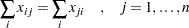
  . The requirement that traffic that flows into each intersection must also flow out is described by the linear equality constraint
 |
In general, roads also have an upper limit on the number of vehicles that can be handled per minute. These limits, denoted  , can be enforced by boundary constraints:
 |
The goal in this problem is to maximize the flow, which is equivalent to maximizing the objective function  , where is
 |
The boundary constraints are
 |
 |
 |
|||
 |
 |
 |
and the flow constraints are
 |
 |
 |
|||
 |
|
 |
|||
 |
|
 |
The three linear equality constraints are linearly dependent. One of them is deleted automatically by the optimization subroutine. The following notation is used in this example:
 |
Even though the NLPCG subroutine is used, any other optimization subroutine would also solve this small problem. The following code finds the maximum flow:
   proc iml;
      title 'Maximum Flow Through a Network';
      start MAXFLOW(x);
         f = x[4] + x[5];
         return(f);
      finish MAXFLOW;

      con = {  0.  0.  0.  0.  0.   .   . ,
              10. 30. 10. 30. 10.   .   . ,
               0.  1. -1.  0. -1.  0.  0. ,
               1.  0.  1. -1.  0.  0.  0. ,
               1.  1.  0. -1. -1.  0.  0. };
      x = j(1,5, 1.);
      optn = {1 3};
      call nlpcg(xres,rc,"MAXFLOW",x,optn,con);
The optimal solution is shown in the following output.
Finding the maximum flow through a network is equivalent to solving a simple linear optimization problem, and for large problems, the LP procedure or the NETFLOW procedure of the SAS/OR product can be used. On the other hand, finding a traffic pattern that minimizes the total delay to move vehicles per minute from node 1 to node 4 includes nonlinearities that need nonlinear optimization techniques. As traffic volume increases, speed decreases. Let  be the travel time on arc
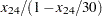
  and assume that the following formulas describe the travel time as decreasing functions of the amount of traffic:
 |
|
 |
|||
 |
|
 |
|||
 |
|
 |
|||
 |
|
 |
|||
 |
|
 |
These formulas use the road capacities (upper bounds), and you can assume that  vehicles per minute have to be moved through the network. The objective is now to minimize
 |
The constraints are
|
|
|
|||
|
|
|
|
|
|
|||
|
|
 |
|||
 |
|
 |
In the following code, the NLPNRR subroutine is used to solve the minimization problem:
   proc iml;
      title 'Minimize Total Delay in Network';
      start MINDEL(x);
         t12 = 5. + .1 * x[1] / (1. - x[1] / 10.);
         t13 = x[2] / (1. - x[2] / 30.);
         t32 = 1. + x[3] / (1. - x[3] / 10.);
         t24 = x[4] / (1. - x[4] / 30.);
         t34 = 5. + .1 * x[5] / (1. - x[5] / 10.);
         f = t12*x[1] + t13*x[2] + t32*x[3] + t24*x[4] + t34*x[5];
         return(f);
      finish MINDEL;

      con = {  0.  0.  0.  0.  0.   .   . ,
              10. 30. 10. 30. 10.   .   . ,
               0.  1. -1.  0. -1.  0.  0. ,
               1.  0.  1. -1.  0.  0.  0. ,
               0.  0.  0.  1.  1.  0.  5. };

      x = j(1,5, 1.);
      optn = {0 3};
      call nlpnrr(xres,rc,"MINDEL",x,optn,con);
The optimal solution is shown in the following output.
The active constraints and corresponding Lagrange multiplier estimates (costs) are shown in the following output.
Copyright © SAS Institute, Inc. All Rights Reserved.