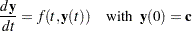
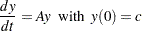
The ODE subroutine performs numerical integration of first-order vector differential equations of the form

The ODE subroutine returns the following values:

r

is a numeric matrix that contains the results of the integration over connected subintervals. The number of columns in is equal to the number of subintervals of integration as defined by the argument . In case of any error in the integration on any subinterval, partial results will not be reported in .

The input arguments to the ODE subroutine are as follows:

"dername"

specifies the name of a module used to evaluate the integrand.

c

specifies an initial value vector for the variable .

t

specifies a sorted vector that describes the limits of integration over connected subintervals. The simplest form of the vector contains only the limits of the integration on one interval. The first component of should contain the initial value, and the second component should be the final value of the independent variable. For more advanced usage of the ODE subroutine, the vector can contain more than two components. The components of the vector must be sorted in ascending order. Two consecutive components of the vector are interpreted as a subinterval. The ODE call reports the final result of integration at the right endpoint of each subinterval. This information is vital if has internal points of discontinuity. To produce accurate solutions, it is essential that you provide the location of these points in the variable , since the continuity of the forcing function is vital to the internal control of error.

h

specifies a numeric vector that contains three components: the minimum allowable step size, hmin; the maximum allowable step size, hmax; and the initial step size to start the integration process, hinit.

"jacobian"

optionally specifies the name of a module that is used to evaluate the Jacobian analytically. The Jacobian is the matrix , with

If the "jacobian" module is not specified, the ODE call uses a finite-difference method to approximate the Jacobian. The keyword for this option is J.

eps

specifies a scalar that indicates the required accuracy. It has a default value of 1E4. The keyword for this option is EPS.

SAS-data-set

(scalar, optional, character, input) a valid predefined SAS data set name that is used to save the successful independent and dependent variables of the integration at each step. The keyword for this option is DATA.

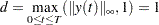
The ODE subroutine is an adaptive, variable order, variable step-size, stiff integrator based on implicit backward-difference methods. see Aiken (1985), Bickart and Picel (1973), Donelson and Hansen (1971), Gaffney (1984), and Shampine (1978). The integrator is an implicit predictor-corrector method that locally attempts to maintain the prescribed precision eps relative to

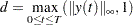As you can see from the expression, this quantity is dynamically updated during the integration process and can help you to understand the validity of the results reported by the subroutine.

Consider the differential equation

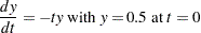The following statements attempt to find the solution at :

  /* Define the integrand */
  start fun(t,y);
      v = -t*y;
      return(v);
  finish;

  /* Call ODE */
  c   = 0.5;
  t   = { 0 1};
  h   = { 1E-12 1 1E-5};
  call ode(r,"FUN",c,t,h);
  print r[format=E21.14];

In this case, the integration is carried out over to give the value of at . The optional parameter eps has not been specified, so it is internally set to 1E4. Also, the optional parameter "jacobian" has not been specified, so finite-difference methods are used to estimate the Jacobian. The accuracy of the answer can be increased by specifying eps. For example, set eps=1E7, as follows:

  /* Define the integrand */
  start fun(t,y);
      v = -t*y;
      return(v);
  finish;

  /* Call ODE */
  c   = 0.5;
  t   = {0 1};
  h   = {1E-12 1. 1E-5};
  call ode(r,"FUN",c,t,h) eps=1E-7;

  print r[format =E21.14];

Compare this value to E and observe that the result is correct through the sixth decimal digit and has an error relative to 1 that is E.

If the solution was desired at 1 and 2 with an accuracy of 1E7, you would use the following statements:

  /* Define the integrand */
  start fun(t,y);
      v = -t*y;
      return(v);
  finish;

  /* Call ODE */
  c   = 0.5;
  t   = { 0 1 2};
  h   = { 1E-12 1. 1E-5};
  call ode(r,"FUN",c,t,h) eps=1E-7;

  print r[format=E21.14];

Note that R contains the solution at in the first column and at in the second column.

Now consider the smoothness of the forcing function . For the purpose of estimating errors, adaptive methods require some degree of smoothness in the function . If this smoothness is not present in over the interior and including the left endpoint of the subinterval, the reported result will not have the desired accuracy. The function must be at least continuous. If the function does not meet this requirement, you should specify the discontinuity as an intermediate point. For example, consider the differential equation

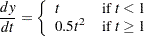To find the solution at , use the following statements:

   /* Define the integrand */
   start fun(t,y);
       if t < 1 then v = t;
       else   v = .5*t*t;
       return(v);
   finish;

   /* Call ODE */
   c   = 0;
   t   = { 0 2};
   h   = { 1E-12 1. 1E-5};
   call ode(r,"FUN",c,t,h) eps = 1E-12;
   print r[format =E21.14];

In the preceding case, the integration is carried out over a single interval, . The optional parameter eps is specified to be 1E12. The optional parameter jacobian is not specified, so finite-difference methods are used to estimate the Jacobian.

Note that the value of R does not have the required accuracy (it should contain a 12 decimal-place representation of 5/3), although no error message is produced. The reason is that the function is not continuous at the point . Even the lowest-order method cannot produce a local reliable error estimate near the point of discontinuity. To avoid this problem, you can create subintervals so that the integration is carried out first over and then over . The following statements implement this method:

   /* Define the integrand */
   start fun(t,y);
       if t < 1 then v = t;
       else          v = .5*t*t;
       return(v);
   finish;

   /* Call ODE */
   c   = 0;
   t   = { 0 1 2};
   h   = { 1E-12 1. 1E-5};
   call ode(r,"FUN",c,t,h) eps=1E-12;
   print r[format=E21.14];

The variable R contains the solutions at both and , and the errors are of the specified order. Although there is no interest in the solution at the point , the advantage of specifying subintervals with no discontinuities is that the function is infinitely differentiable in each subinterval.

When is continuous, the ODE subroutine can compute the integration to the specified precision, even if the function is defined piecewise. Consider the differential equation

The following statements finds the solution at : Since the function is continuous, the requirements for error control are satisfied.

   /* Define the integrand */
   start fun(t,y);
       if t < 1 then v = t;
       else          v = t*t;
       return(v);
   finish;

   /* Call ODE */
   c   = 0.5;
   t   = { 0 2};
   h   = { 1E-12 1. 1E-5};
   call ode(r,"FUN",c,t,h) eps=1E-12;
   print r[format=E21.14];

This example compares the ODE call to an eigenvalue decomposition for stiff-linear systems. In the problem

where is a symmetric constant matrix, the solution can be written in terms of the eigenvalue decomposition, as follows:

where is the matrix of eigenvectors and is a diagonal matrix with the eigenvalues on its diagonal.

The following statements produce two solutions, one by using the ODE call and the other by using the eigenvalue decomposition:

    /* Define the integrand */
    start fun(t,x) global(a,count);
       count = count+1;
       v = a*x;
       return(v);
    finish;

    /* Define the Jacobian */
    start jac(t,x) global(a);
       v = a;
       return(v);
    finish;

    a = {-1000 -1 -2 -3,
            -1 -2  3 -1,
            -2  3 -4 -3,
            -3 -1 -3 -5 };

    /* Call ODE */
    count = 0;
    t = { 0 1 2};
    h = {1E-12  1 1E-5};
    eps = 1E-9;
    c = {1, 0, 0, 0 };
    call ode(z,"FUN",c,t,h)  eps=eps j="JAC";
    print z[format=E21.14];

     print count;

   /* Do the eigenvalue decomposition */
   start eval(t) global(d,u,c);
      v = u*diag(exp(d*t))*u`*c;
      return(v);
   finish;

   call eigen(d,u,a);
   free z1;
   do i = 1 to nrow(t)*ncol(t)-1;
     z1 = z1 || (eval(t[i+1]));
   end;
   print z1[format=E21.14];

The question now is whether or not this is an E result. Note that for the problem

with the 1E6 result, the ODE call should attempt to maintain an accuracy of 1E9 relative to 1. Therefore, the 1E6 result should have almost three correct decimal places. At , the first component of is 6.58597048842310E06, while its more accurate value is 6.58580950203220E06, showing an E error.

The ODE subroutine can fail for problems with unusual qualitative properties, such as finite escape time in the interval of integration (that is, the solution goes towards infinity at some finite time). In such cases, try testing with different subintervals and different levels of accuracy to gain some qualitative information about the behavior of the solution of the differential equation.