| Language Reference |
| BSPLINE Function |
The BSPLINE function computes a B-spline basis. The arguments to the BSPLINE function are as follows:
- x
is an
 or
or  numeric vector.
 - d
is a nonnegative numeric scalar value that specifies the degree of the B-spline. The order of a B-spline is one greater than the degree.
- k
is a numeric vector of size
 that contains the B-spline knots or a scalar that denotes the number of interior knots. When
  , the elements of the knot vector must be nondecreasing,
  for
for  .
. - i
is an optional argument that specifies the number of interior knots when
 and
and  contains a missing value. In this case the BSPLINE function constructs a vector of knots as follows: If
  and
and  are the smallest and largest value in the
  vector, then interior knots are placed at
In addition,
 exterior knots are placed under and max(,1) exterior knots are placed over . The exterior knots are evenly spaced and start at
  1E
1E 12 and
  1E12. In this case the BSPLINE function returns a matrix with
  rows and
  columns.
The BSPLINE function computes B-splines of degree . Suppose that  denotes the
  th B-spline of degree in the knot sequence
  . DeBoor (1981) defines the splines based on the following relationships:
 |
and for 
 |
 |
 |
|||
 |
|
 |
Note that DeBoor (1981) expresses B-splines in terms of order rather than degree; in his notation  . B-splines have many interesting properties, including the following:

The sequence
 is positive on
  knots and zero elsewhere.
 The B-spline
is a piecewise polynomial of at most pieces. If
 , then
  .
.
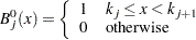
See DeBoor (1981) for more details. The BSPLINE function defines B-splines of degree 0 as nonzero if  .
.
A typical knot vector for calculating B-splines consists of exterior knots smaller than the smallest data value, and  exterior knots larger than the largest data value. The remaining knots are the interior knots.
For example, the following statements creates a B-spline basis with three interior knots. The BSPLINE function returns a matrix with  columns, shown in Figure 23.47.
x     = {2.5 3 4.5 5.1};     /* data range is [2.5, 5.1] */
knots = {0 1 2 3 4 5 6 7 8}; /* three interior knots at x=3, 4, 5 */
bsp = bspline(x, 3, knots);
print bsp[format=best7.];
If you pass an vector of data values, you can also rely on the BSPLINE function to compute a knot vector for you. For example, the following statements compute B-splines of degree 2 based on four equally spaced interior knots:
n = 15;
x = ranuni(J(n, 1, 45));
bsp2 = bspline(x, 2, ., 4);
print bsp2[format=8.3];
The resulting matrix is shown in Figure 23.47.
| bsp2 | ||||||
|---|---|---|---|---|---|---|
| 0.000 | 0.104 | 0.748 | 0.147 | 0.000 | 0.000 | 0.000 |
| 0.000 | 0.000 | 0.000 | 0.286 | 0.684 | 0.030 | 0.000 |
| 0.000 | 0.000 | 0.000 | 0.000 | 0.000 | 0.517 | 0.483 |
| 0.000 | 0.000 | 0.000 | 0.217 | 0.725 | 0.058 | 0.000 |
| 0.000 | 0.000 | 0.239 | 0.713 | 0.048 | 0.000 | 0.000 |
| 0.000 | 0.000 | 0.000 | 0.446 | 0.553 | 0.002 | 0.000 |
| 0.000 | 0.000 | 0.394 | 0.600 | 0.006 | 0.000 | 0.000 |
| 0.000 | 0.000 | 0.000 | 0.000 | 0.064 | 0.729 | 0.207 |
| 0.000 | 0.389 | 0.604 | 0.007 | 0.000 | 0.000 | 0.000 |
| 0.000 | 0.000 | 0.000 | 0.000 | 0.000 | 0.500 | 0.500 |
| 0.000 | 0.000 | 0.000 | 0.000 | 0.210 | 0.728 | 0.062 |
| 0.000 | 0.000 | 0.014 | 0.639 | 0.347 | 0.000 | 0.000 |
| 0.000 | 0.001 | 0.546 | 0.453 | 0.000 | 0.000 | 0.000 |
| 0.500 | 0.500 | 0.000 | 0.000 | 0.000 | 0.000 | 0.000 |
| 0.304 | 0.672 | 0.024 | 0.000 | 0.000 | 0.000 | 0.000 |
Copyright © SAS Institute, Inc. All Rights Reserved.