Time Series Analysis and Examples: Spectral Analysis

Time Series Analysis and Examples

Spectral Analysis

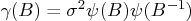
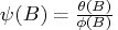
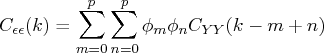
The autocovariance function of the random variable is defined as

$c_{yy}(k) = {\rm e}(y_{t+k} y_t)$

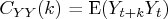
where ${\rm e}y_t = 0$ . When the real valued process

is stationary and its autocovariance is absolutely summable, the population spectral density function is obtained by using the Fourier transform of the autocovariance function

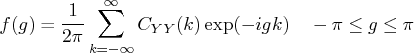
$f(g) = \frac{1}{2 \pi} \sum_{k = -\infty}^{\infty} c_{yy}(k) \exp(-igk) \hspace*{0.15in} -\pi \leq g \leq \pi$

where $i=\sqrt{-1}$ and $c_{yy}(k)$ is the autocovariance function such that $\sum_{k = -\infty}^{\infty} | c_{yy}(k)| \lt \infty$ .

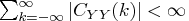
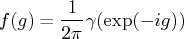
Consider the autocovariance generating function

$\gamma(z) = \sum_{k = -\infty}^{\infty} c_{yy}(k) z^k$

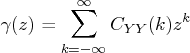
where $c_{yy}(k) = c_{yy}(-k)$ and

is a complex scalar. The spectral density function can be represented as

$f(g) = \frac{1}{2 \pi} \gamma(\exp(-ig))$

The stationary ARMA(

) process is denoted

$\phi(b) y_t = \theta(b) \epsilon_t \hspace*{0.15in} \epsilon_t \sim(0,\sigma^2)$

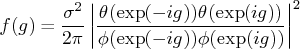
where $\phi(b)$ and $\theta(b)$ do not have common roots. Note that the autocovariance generating function of the linear process $y_t = \psi(b)\epsilon_t$ is given by

$\gamma(b) = \sigma^2\psi(b)\psi(b^{-1})$

For the ARMA(

) process, $\psi(b) = \frac{\theta(b)}{\phi(b)}$ . Therefore, the spectral density function of the stationary ARMA(

) process becomes

$f(g) = \frac{\sigma^2}{2\pi}|\frac{\theta(\exp(-ig)) \theta(\exp(ig))}{\phi(\exp(-ig))\phi(\exp(ig))}|^2$

The spectral density function of a white noise is a constant.

$f(g) = \frac{\sigma^2}{2\pi}$

The spectral density function of the AR(1) process $(\phi(b) = 1-\phi_1 b)$ is given by

$f(g) = \frac{\sigma^2}{2\pi(1-\phi_1 \cos(g) + \phi_1^2)}$

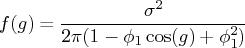
The spectrum of the AR(1) process has its minimum at

and its maximum at $g=+-\pi$ if $\phi_1 \lt 0$ , while the spectral density function attains its maximum at

and its minimum at $g=+-\pi$ , if $\phi_1\gt$ . When the series is positively autocorrelated, its spectral density function is dominated by low frequencies. It is interesting to observe that the spectrum approaches $\frac{\sigma^2}{4\pi}\frac{1}{1-\cos(g)}$ as $\phi_1arrow 1$ . This relationship shows that the series is difference-stationary if its spectral density function has a remarkable peak near 0.

The spectrum of AR(2) process 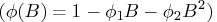$(\phi(b)=1-\phi_1 b-\phi_2 b^2)$ equals

$f(g) = \frac{\sigma^2}{2\pi}\frac{1} {\{-4\phi_2[\cos(g)+\frac{\phi_1(1-\phi_2)} {4\phi_2}]^2 + \frac{(1+\phi_2)^2(4\phi_2 + \phi_1^2)} {4\phi_2}\}}$

Refer to Anderson (1971) for details of the characteristics of this spectral density function of the AR(2) process.

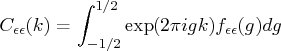
In practice, the population spectral density function cannot be computed. There are many ways of computing the sample spectral density function. The TSBAYSEA and TSMLOCAR subroutines compute the power spectrum by using AR coefficients and the white noise variance.

The power spectral density function of is derived by using the Fourier transformation of $c_{yy}(k)$ .

$f_{yy}(g) = \sum_{k=-\infty}^\infty \exp(-2\pi igk)c_{yy}(k), \hspace*{.25in} -\frac{1}2\leq g \leq\frac{1}2$

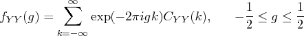
where $i=\sqrt{-1}$ and

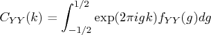
denotes frequency. The autocovariance function can also be written as

$c_{yy}(k) = \int_{-1/2}^{1/2} \exp(2\pi igk)f_{yy}(g)dg$

Consider the following stationary AR(

) process:

$y_t - \sum_{i=1}^p \phi_i y_{t-i} = \epsilon_t$

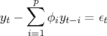
where $\epsilon_t$ is a white noise with mean zero and constant variance $\sigma^2$ .

The autocovariance function of white noise $\epsilon_t$ equals

$c_{\epsilon\epsilon}(k) = \delta_{k0}\sigma^2$

where $\delta_{k0}=1$ if

; otherwise, $\delta_{k0}=0$ . Therefore, the power spectral density of the white noise is $f_{\epsilon\epsilon}(g) = \sigma^2$ , $-\frac{1}2\leq g \leq\frac{1}2$ . Note that, with $\phi_0 = -1$ ,

$c_{\epsilon\epsilon}(k) = \sum_{m=0}^p \sum_{n=0}^p \phi_m\phi_n c_{yy}(k-m+n)$

Using the following autocovariance function of

$c_{yy}(k) = \int_{-1/2}^{1/2} \exp(2\pi igk)f_{yy}(g)dg$

the autocovariance function of the white noise is denoted as

$c_{\epsilon\epsilon}(k) & = & \sum_{m=0}^p \sum_{n=0}^p \phi_m\phi_n \int_{-1/... ...^{1/2} \exp(2\pi igk) \,| 1-\sum_{m=1}^p \phi_m\exp(-2\pi igm)|^2 f_{yy}(g)dg$

On the other hand, another formula of the $c_{\epsilon\epsilon}(k)$ gives

$c_{\epsilon\epsilon}(k) = \int_{-1/2}^{1/2} \exp(2\pi igk) f_{\epsilon\epsilon}(g)dg$

Therefore,

$f_{\epsilon\epsilon}(g) = | 1-\sum_{m=1}^p \phi_m\exp(-2\pi igm) |^2 f_{yy}(g)$

Since $f_{\epsilon\epsilon}(g) = \sigma^2$ , the rational spectrum of

$f_{yy}(g) = \frac{\sigma^2} {| 1-\sum_{m=1}^p \phi_m\exp(-2\pi igm)|^2}$

To compute the power spectrum, estimated values of white noise variance $\hat{\sigma}^2$ and AR coefficients $\hat{\phi}_m$ are used. The order of the AR process can be determined by using the minimum AIC procedure.

Top of Page