Time Series Analysis and Examples: Computational Details

Time Series Analysis and Examples

Computational Details

Least Squares and Householder Transformation

Consider the univariate AR(

) process

$y_t = \alpha_0 + \sum_{i=1}^p \alpha_i y_{t-i} + \epsilon_t$

Define the design matrix

${x}= [1 & y_p & ... & y_1 \ \vdots & \vdots & \ddots & \vdots \ 1 & y_{t-1} & ... & y_{t-p} ]$

Let ${y}= (y_{p+1}, ... ,y_n)^'$ . The least squares estimate, $\hat{{a}}=({x}^'{x})^{-1}{x}^'{y}$ , is the approximation to the maximum likelihood estimate of ${a}=(\alpha_0,\alpha_1, ... ,\alpha_p)$ if $\epsilon_t$ is assumed to be Gaussian error disturbances. Combining

and

${z}= [{x}\,\vdots\,{y}]$

the

matrix can be decomposed as

${z}= {q}{u}= {q}[{{r}}& {w}_1 \ 0 & {w}_2 ]$

where

is an orthogonal matrix and

is an upper triangular matrix, ${w}_1 = (w_1, ... ,w_{p+1})^'$ , and ${w}_2 = (w_{p+2},0, ... ,0)^'$ .

${q}^'{y}= [w_1 \ w_2 \ \vdots \ w_{t-p} ]$

The least squares estimate that uses Householder transformation is computed by solving the linear system

${{r}}{a}= {w}_1$

The unbiased residual variance estimate is

$\hat{\sigma}^2 = \frac{1}{t-p} \sum_{i=p+2}^{t-p} w_i^2 = \frac{w_{p+2}^2}{t-p}$

and

${\rm aic}=(t-p)\log(\hat{\sigma}^2) + 2(p+1)$

In practice, least squares estimation does not require the orthogonal matrix

. The TIMSAC subroutines compute the upper triangular matrix without computing the matrix

Bayesian Constrained Least Squares

Consider the additive time series model

$y_t = t_t + s_t + \epsilon_t,\hspace*{.25in}\epsilon_t\sim n(0,\sigma^2)$

Practically, it is not possible to estimate parameters ${a}= (t_1, ... ,t_t,s_1, ... ,s_t)^'$ , since the number of parameters exceeds the number of available observations. Let $\nabla_l^m$ denote the seasonal difference operator with seasons and degree of ; that is, $\nabla_l^m = (1-b^l)^m$ . Suppose that . Some constraints on the trend and seasonal components need to be imposed such that the sum of squares of $\nabla^k t_t$ , $\nabla_l^m s_t$ , and $(\sum_{i=0}^{l-1} s_{t-i})$ is small. The constrained least squares estimates are obtained by minimizing

$\sum_{t=1}^t \{(y_t-t_t-s_t)^2 + d^2[s^2(\nabla^k t_t)^2 + (\nabla_l^m s_t)^2 + z^2(s_t+ ... +s_{t-l+1})^2]\}$

Using matrix notation,

$({y}-{m}{a})^'({y}-{m}{a}) + ({a}-{a}_0)^'{d}^'{d}({a}-{a}_0)$

where ${m}= [{i}_t\,\vdots\,{i}_t]$ , ${y}= (y_1, ... , y_t)^'$ , and ${a}_0$ is the initial guess of

. The matrix

is a

control matrix in which structure varies according to the order of differencing in trend and season.

${d}= d [{e}_m & 0 \ z{f}& 0 \ 0 & s{g}_k ]$

where

${e}_m & = & {c}_m\otimes{i}_l,\hspace*{.25in} m=1,2,3 \ {f}& = & [1 & 0 & ...... ...s & \ddots & \ddots & \ddots & 0 \ 0 & ... & 0 & -1 & 3 & -3 & 1 ]_{tx t}$

The

matrix ${c}_m$ has the same structure as the matrix ${g}_m$ , and ${i}_l$ is the

identity matrix. The solution of the constrained least squares method is equivalent to that of maximizing the function

$l({a}) = \exp\{-\frac{1}{2\sigma^2}({y}-{m}{a})^'({y}-{m}{a})\} \exp\{-\frac{1}{2\sigma^2}({a}-{a}_0)^'{d}^'{d}({a}-{a}_0)\}$

Therefore, the PDF of the data

$f({y}|\sigma^2,{a}) = (\frac{1}{2\pi})^{t/2} (\frac{1}{\sigma})^t \exp\{-\frac{1}{2\sigma^2}({y}-{m}{a})^'({y}-{m}{a})\}$

The prior PDF of the parameter vector

$\pi({a}|{d},\sigma^2,{a}_0) = (\frac{1}{2\pi})^t (\frac{1}{\sigma})^{2t}|{d}^'{d}| \exp\{-\frac{1}{2\sigma^2}({a}-{a}_0)^'{d}^'{d}({a}-{a}_0)\}$

When the constant

is known, the estimate $\hat{{a}}$ of

is the mean of the posterior distribution, where the posterior PDF of the parameter

is proportional to the function

. It is obvious that $\hat{{a}}$ is the minimizer of $\vert{g}({a}| d)\vert^2 = (\tilde{{y}}-\tilde{{d}}{a})^'(\tilde{{y}}-\tilde{{d}}{a})$ , where

$\tilde{{y}} = [{y}\ {d}{a}_0 ]$

$\tilde{{d}} = [{m}\ {d} ]$

The value of

is determined by the minimum ABIC procedure. The ABIC is defined as

${\rm abic} = t\log[\frac{1}t\vert{g}({a}| d)\vert^2] + 2\{\log[\det({d}^'{d}+{m}^'{m})] - \log[\det({d}^'{d})]\}$

State Space and Kalman Filter Method

In this section, the mathematical formulas for state space modeling are introduced. The Kalman filter algorithms are derived from the state space model. As an example, the state space model of the TSDECOMP subroutine is formulated.

Define the following state space model:

${x}_t &=& {f}{x}_{t-1} + {g}{w}_t \ y_t &=& {h}_t{x}_t + \epsilon_t$

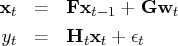
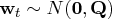
where $\epsilon_t\sim n(0,\sigma^2)$ and ${w}_t\sim n(0,{q})$ . If the observations,

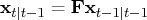
, and the initial conditions, ${x}_{0|}$ and ${p}_{0|}$ , are available, the one-step predictor $({x}_{t| t-1})$ of the state vector ${x}_t$ and its mean square error (MSE) matrix ${p}_{t| t-1}$ are written as

${x}_{t| t-1} = {f}{x}_{t-1| t-1}$

${p}_{t| t-1} = {f}{p}_{t-1| t-1}{f}^' + {g}{q}{g}^'$

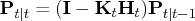
Using the current observation, the filtered value of ${x}_t$ and its variance ${p}_{t| t}$ are updated.

${x}_{t| t} = {x}_{t| t-1} + {k}_t e_t$

${p}_{t| t} = ({i}- {k}_t {h}_t){p}_{t| t-1}$

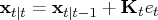
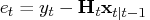
where $e_t = y_t - {h}_t{x}_{t| t-1}$ and ${k}_t = {p}_{t| t-1}{h}^'_t[{h}_t {p}_{t| t-1}{h}^'_t + \sigma^2{i}]^{-1}$ . The log-likelihood function is computed as

$\ell = -\frac{1}2\sum_{t=1}^t \log(2\pi v_{t| t-1}) - \sum_{t=1}^t \frac{e_t^2}{2v_{t| t-1}}$

where $v_{t| t-1}$ is the conditional variance of the one-step prediction error

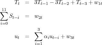
Consider the additive time series decomposition

$y_t = t_t + s_t + t\!d_t + u_t + {x}^'_t\beta_t + \epsilon_t$

where ${x}_t$ is a

regressor vector and $\beta_t$ is a

time-varying coefficient vector. Each component has the following constraints:

$\nabla^k t_t & = & w_{1t},\hspace*{.25in}w_{1t}\sim n(0,\tau_1^2) \ \nabla_l^m... ...m_{i=1}^6 \gamma_{it}(t\!d_t(i)-t\!d_t(7)) \ \gamma_{it} & = & \gamma_{i,t-1}$