| Time Series Analysis and Examples |
Multivariate Time Series Analysis
The subroutines TSMULMAR, TSMLOMAR, and TSPRED analyze multivariate time series. The periodic AR model, TSPEARS, can also be estimated by using a vector AR procedure, since the periodic AR series can be represented as the covariance-stationary vector autoregressive model.
The stationary vector AR model is estimated and the order of the model (or each variable) is automatically determined by the minimum AIC procedure. The stationary vector AR model is written
The TSMULMAR subroutine estimates the instantaneous response model. The VAR coefficients are computed by using the relationship between the VAR and instantaneous models.
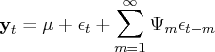
The general VARMA model can be transformed as an infinite-order MA process under certain conditions.
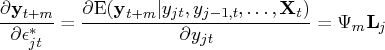
The MSE of the ![]() -step prediction is computed as
-step prediction is computed as
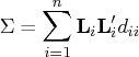
![\sum_{i=1}^n d_{ii} [ {l}_i {l}^'_i + \psi_1 {l}_i {l}^'_i \psi^'_1 + ... + \psi_{m-1} {l}_i {l}^'_i \psi^'_{m-1} ]](images/timeseriesexpls_timeseriesexplseq217.gif)
The nonstationary multivariate series can be analyzed by the TSMLOMAR subroutine. The estimation and model identification procedure is analogous to the univariate nonstationary procedure, which is explained in the section "Nonstationary Time Series".
A time series ![]() is periodically correlated
with period
is periodically correlated
with period ![]() if
if ![]() and
and ![]() .
Let
.
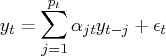
Let ![]() be autoregressive of period
be autoregressive of period ![]() with AR orders
with AR orders ![]() - that is,
- that is,
The TSPRED subroutine computes the one-step or multistep forecast of the multivariate ARMA model if the ARMA parameter estimates are provided. In addition, the subroutine TSPRED produces the (intermediate and permanent) impulse response function and performs forecast error variance decomposition for the vector AR model.
Copyright © 2009 by SAS Institute Inc., Cary, NC, USA. All rights reserved.