| Time Series Analysis and Examples |
Nonstationary Time Series
The subroutines TSMLOCAR, TSMLOMAR, and TSTVCAR are used to analyze nonstationary time series models. The AIC statistic is extensively used to analyze the locally stationary model.
Locally Stationary AR Model
When the time series is nonstationary, the TSMLOCAR (univariate) and TSMLOMAR (multivariate) subroutines can be employed. The whole span of the series is divided into locally stationary blocks of data, and then the TSMLOCAR and TSMLOMAR subroutines estimate a stationary AR model by using the least squares method on this stationary block. The homogeneity of two different blocks of data is tested by using the AIC.
Given a set of data ![]() , the data can be
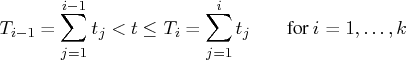
divided into
, the data can be
divided into ![]() blocks of sizes
blocks of sizes ![]() , where
, where
![]() , and
, and ![]() and
and ![]() are unknown.
The locally stationary model is fitted to the data
are unknown.
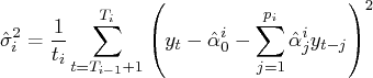
The locally stationary model is fitted to the data
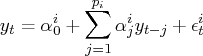
![\ell = -\frac{1}2\sum_{i=1}^k [ t_i\log(2 \pi \sigma_i^2) + \frac{1}{\sigma_i^... ...1}^{t_i} ( y_t - \alpha_0^i - \sum_{j=1}^{p_i} \alpha_j^i y_{t-j} )^2 ]](images/timeseriesexpls_timeseriesexplseq159.gif)
![\ell^* = - \frac{t}2[1 + \log(2 \pi)] - \frac{1}2 \sum_{i=1}^k t_i \log(\hat{\sigma}_i^2)](images/timeseriesexpls_timeseriesexplseq163.gif)
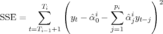
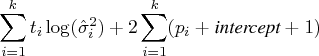
The AIC for the locally stationary model over the pooled data is written as
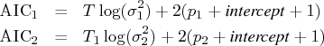
When the two data sets are pooled and estimated
over the pooled data set, ![]() ,
the AIC of the pooled model is
,
the AIC of the pooled model is
Decision
- If
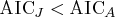 , switch to the new model,
since there is a change in the structure of the time series.
, switch to the new model,
since there is a change in the structure of the time series.
- If
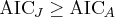 , pool the two data sets,
since two data sets are considered to be homogeneous.
, pool the two data sets,
since two data sets are considered to be homogeneous.
Time-Varying AR Coefficient Model
Another approach to nonstationary time series, especially those that are nonstationary in the covariance, is time-varying AR coefficient modeling. When the time series is nonstationary in the covariance, the problem in modeling this series is related to an efficient parameterization. It is possible for a Bayesian approach to estimate the model with a large number of implicit parameters of the complex structure by using a relatively small number of hyperparameters.
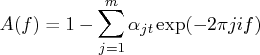
The TSTVCAR subroutine uses smoothness priors by imposing stochastically perturbed difference equation constraints on each AR coefficient and frequency response function. The variance of each AR coefficient distribution constitutes a hyperparameter included in the state space model. The likelihood of these hyperparameters is computed by the Kalman filter recursive algorithm.
The time-varying AR coefficient model is written
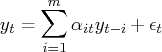

Using a state space representation, the model is
![{x}_t & = & (\alpha_{1t}, ... ,\alpha_{mt}, ... , \alpha_{1,t-k+1}, ... ,\alph... ...{w}_t \ \epsilon_t ] & \sim & n (0, [ \tau^2{i}& 0 \ 0 & \sigma^2 ] )](images/timeseriesexpls_timeseriesexplseq192.gif)
Copyright © 2009 by SAS Institute Inc., Cary, NC, USA. All rights reserved.