Robust Regression Examples: Example 9.5: Stackloss Data

Robust Regression Examples

Example 9.5: Stackloss Data

The following example analyzes the three regressors of Brownlee (1965) stackloss data. By default, the MVE subroutine tries only 2000 randomly selected subsets in its search. There are, in total, 5985 subsets of 4 cases out of 21 cases. Here is the code:

  
    title2 "***MVE for Stackloss Data***"; 
    title3 "*** Use All Subsets***"; 
       a = aa[,2:4]; 
       optn = j(9,1,.); 
       optn[1]= 2;              /* ipri */ 
       optn[2]= 1;              /* pcov: print COV */ 
       optn[3]= 1;              /* pcor: print CORR */ 
       optn[5]= -1;             /* nrep: use all subsets */ 
    call mve(sc,xmve,dist,optn,a);

Output 9.5.1 of the output shows the classical scatter and correlation matrix.

Output 9.5.1: Some Simple Statistics

Minimum Volume Ellipsoid (MVE) Estimation

Consider Ellipsoids Containing 12 Cases.

Classical Covariance Matrix
	VAR1	VAR2	VAR3
VAR1	84.057142857	22.657142857	24.571428571
VAR2	22.657142857	9.9904761905	6.6214285714
VAR3	24.571428571	6.6214285714	28.714285714

Classical Correlation Matrix
	VAR1	VAR2	VAR3
VAR1	1	0.781852333	0.5001428749
VAR2	0.781852333	1	0.3909395378
VAR3	0.5001428749	0.3909395378	1

Classical Mean
VAR1	60.428571429
VAR2	21.095238095
VAR3	86.285714286

Output 9.5.2 shows the results of the optimization (complete subset sampling).

Output 9.5.2: Iteration History

***MVE for Stackloss Data***

Subset	Singular	Best Criterion	Percent
1497	22	253.312431	25
2993	46	224.084073	50
4489	77	165.830053	75
5985	156	165.634363	100

Observations of Best Subset
7	10	14	20

Initial MVE Location Estimates
VAR1	58.5
VAR2	20.25
VAR3	87

Initial MVE Scatter Matrix
	VAR1	VAR2	VAR3
VAR1	34.829014749	28.413143611	62.32560534
VAR2	28.413143611	38.036950318	58.659393261
VAR3	62.32560534	58.659393261	267.63348175

Output 9.5.3 shows the optimization results after local improvement.

Output 9.5.3: Table of MVE Results

***MVE for Stackloss Data***

Robust MVE Location Estimates
VAR1	56.705882353
VAR2	20.235294118
VAR3	85.529411765

Robust MVE Scatter Matrix
	VAR1	VAR2	VAR3
VAR1	23.470588235	7.5735294118	16.102941176
VAR2	7.5735294118	6.3161764706	5.3676470588
VAR3	16.102941176	5.3676470588	32.389705882

Eigenvalues of Robust Scatter Matrix
VAR1	46.597431018
VAR2	12.155938483
VAR3	3.423101087

Robust Correlation Matrix
	VAR1	VAR2	VAR3
VAR1	1	0.6220269501	0.5840361335
VAR2	0.6220269501	1	0.375278187
VAR3	0.5840361335	0.375278187	1

Output 9.5.4 presents a table containing the classical Mahalanobis distances, the robust distances, and the weights identifying the outlying observations (that is, the leverage points when explaining with these three regressor variables).

Output 9.5.4: Mahalanobis and Robust Distances

***MVE for Stackloss Data***

Classical Distances and Robust (Rousseeuw) Distances
Unsquared Mahalanobis Distance and
Unsquared Rousseeuw Distance of Each Observation
N	Mahalanobis Distances	Robust Distances	Weight
1	2.253603	5.528395	0
2	2.324745	5.637357	0
3	1.593712	4.197235	0
4	1.271898	1.588734	1.000000
5	0.303357	1.189335	1.000000
6	0.772895	1.308038	1.000000
7	1.852661	1.715924	1.000000
8	1.852661	1.715924	1.000000
9	1.360622	1.226680	1.000000
10	1.745997	1.936256	1.000000
11	1.465702	1.493509	1.000000
12	1.841504	1.913079	1.000000
13	1.482649	1.659943	1.000000
14	1.778785	1.689210	1.000000
15	1.690241	2.230109	1.000000
16	1.291934	1.767582	1.000000
17	2.700016	2.431021	1.000000
18	1.503155	1.523316	1.000000
19	1.593221	1.710165	1.000000
20	0.807054	0.675124	1.000000
21	2.176761	3.657281	0

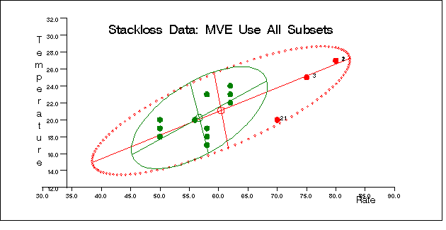
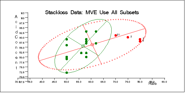
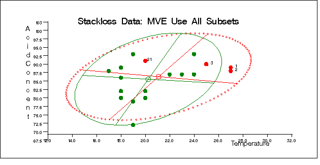
The following specification generates three bivariate plots of the classical and robust tolerance ellipsoids. They are shown in Figure 9.5.5, Figure 9.5.6, and Figure 9.5.7, one plot for each pair of variables.

  
       optn = j(9,1,.); optn[5]= -1; 
       vnam = { "Rate", "Temperature", "AcidConcent" }; 
       filn = "stlmve"; 
       titl = "Stackloss Data: Use All Subsets"; 
    call scatmve(2,optn,.9,a,vnam,titl,1,filn);

Output 9.5.5: Stackloss Data: Rate vs. Temperature (MVE)

Output 9.5.6: Stackloss Data: Rate vs. Acid Concentration (MVE)

Output 9.5.7: Stackloss Data: Temperature vs. Acid Concentration (MVE)

You can also use the MCD method for the stackloss data as follows:

  
   title2 "***MCD for Stackloss Data***"; 
   title3 "*** Use 500 Random Subsets***"; 
   a = aa[,2:4]; 
   optn = j(8,1,.); 
   optn[1]= 2;              /* ipri */ 
   optn[2]= 1;              /* pcov: print COV */ 
   optn[3]= 1;              /* pcor: print CORR */ 
   optn[5]= -1 ;            /* nrep: use all subsets */ 
   CALL MCD(sc,xmcd,dist,optn,a);

The optimization results are displayed in Output 9.5.8. The reweighted results are displayed in Output 9.5.9.

Output 9.5.8: MCD Results of Optimization

***MCD for Stackloss Data***

*** Use 500 Random Subsets***

MCD Location Estimate
VAR1	VAR2	VAR3
59.5	20.833333333	87.333333333

MCD Scatter Matrix Estimate
	VAR1	VAR2	VAR3
VAR1	5.1818181818	4.8181818182	4.7272727273
VAR2	4.8181818182	7.6060606061	5.0606060606
VAR3	4.7272727273	5.0606060606	19.151515152

MCD Correlation Matrix
	VAR1	VAR2	VAR3
VAR1	1	0.7674714142	0.4745347313
VAR2	0.7674714142	1	0.4192963398
VAR3	0.4745347313	0.4192963398	1

Consistent Scatter Matrix
	VAR1	VAR2	VAR3
VAR1	8.6578437815	8.0502757968	7.8983838007
VAR2	8.0502757968	12.708297013	8.4553211199
VAR3	7.8983838007	8.4553211199	31.998580526

Output 9.5.9: Final Reweighted MCD Results

***MCD for Stackloss Data***

*** Use 500 Random Subsets***

Reweighted Location Estimate
VAR1	VAR2	VAR3
59.5	20.833333333	87.333333333

Reweighted Scatter Matrix
	VAR1	VAR2	VAR3
VAR1	5.1818181818	4.8181818182	4.7272727273
VAR2	4.8181818182	7.6060606061	5.0606060606
VAR3	4.7272727273	5.0606060606	19.151515152

Eigenvalues
VAR1	VAR2	VAR3
23.191069268	7.3520037086	1.3963209628

Reweighted Correlation Matrix
	VAR1	VAR2	VAR3
VAR1	1	0.7674714142	0.4745347313
VAR2	0.7674714142	1	0.4192963398
VAR3	0.4745347313	0.4192963398	1

The MCD robust distances and outlying diagnostic are displayed in Output 9.5.10. MCD identifies more leverage points than MVE.

Output 9.5.10: MCD Robust Distances

***MCD for Stackloss Data***

*** Use 500 Random Subsets***

Classical Distances and Robust (Rousseeuw) Distances
Unsquared Mahalanobis Distance and
Unsquared Rousseeuw Distance of Each Observation
N	Mahalanobis Distances	Robust Distances	Weight
1	2.253603	12.173282	0
2	2.324745	12.255677	0
3	1.593712	9.263990	0
4	1.271898	1.401368	1.000000
5	0.303357	1.420020	1.000000
6	0.772895	1.291188	1.000000
7	1.852661	1.460370	1.000000
8	1.852661	1.460370	1.000000
9	1.360622	2.120590	1.000000
10	1.745997	1.809708	1.000000
11	1.465702	1.362278	1.000000
12	1.841504	1.667437	1.000000
13	1.482649	1.416724	1.000000
14	1.778785	1.988240	1.000000
15	1.690241	5.874858	0
16	1.291934	5.606157	0
17	2.700016	6.133319	0
18	1.503155	5.760432	0
19	1.593221	6.156248	0
20	0.807054	2.172300	1.000000
21	2.176761	7.622769	0

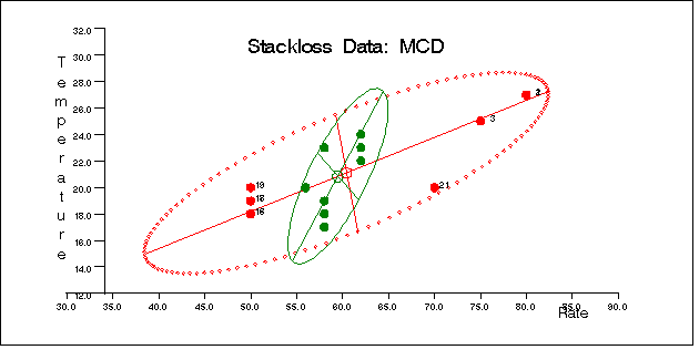
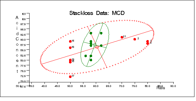
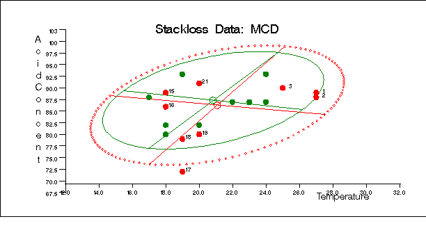
Similarly, you can use the SCATMCD routine to generate three bivariate plots of the classical and robust tolerance ellipsoids, one plot for each pair of variables. Here is the code:

  
       optn = j(9,1,.); optn[5]= -1; 
       vnam = { "Rate", "Temperature", "AcidConcent" }; 
       filn = "stlmcd"; 
       titl = "Stackloss Data: Use All Subsets"; 
    call scatmcd(2,optn,.9,a,vnam,titl,1,filn);

Figure 9.5.11, Figure 9.5.12, and Figure 9.5.13 display these plots.

Output 9.5.11: Stackloss Data: Rate vs. Temperature (MCD)

Output 9.5.12: Stackloss Data: Rate vs. Acid Concentration (MCD)

Output 9.5.13: Stackloss Data: Temperature vs. Acid Concentration (MCD)

Top of Page