Robust Regression Examples: Example 9.6: Hawkins-Bradu-Kass Data

Robust Regression Examples

Example 9.6: Hawkins-Bradu-Kass Data

The first 14 observations of the following data set (see Hawkins, Bradu, and Kass 1984) are leverage points; however, only observations 12, 13, and 14 have large $h_{ii}$ , and only observations 12 and 14 have large values.

  
    title "Hawkins, Bradu, Kass (1984) Data"; 
       aa = { 1  10.1  19.6  28.3   9.7, 
              2   9.5  20.5  28.9  10.1, 
              3  10.7  20.2  31.0  10.3, 
              4   9.9  21.5  31.7   9.5, 
              5  10.3  21.1  31.1  10.0, 
              6  10.8  20.4  29.2  10.0, 
              7  10.5  20.9  29.1  10.8, 
              8   9.9  19.6  28.8  10.3, 
              9   9.7  20.7  31.0   9.6, 
             10   9.3  19.7  30.3   9.9, 
             11  11.0  24.0  35.0  -0.2, 
             12  12.0  23.0  37.0  -0.4, 
             13  12.0  26.0  34.0   0.7, 
             14  11.0  34.0  34.0   0.1, 
             15   3.4   2.9   2.1  -0.4, 
             16   3.1   2.2   0.3   0.6, 
             17   0.0   1.6   0.2  -0.2, 
             18   2.3   1.6   2.0   0.0, 
             19   0.8   2.9   1.6   0.1, 
             20   3.1   3.4   2.2   0.4, 
             21   2.6   2.2   1.9   0.9, 
             22   0.4   3.2   1.9   0.3, 
             23   2.0   2.3   0.8  -0.8, 
             24   1.3   2.3   0.5   0.7, 
             25   1.0   0.0   0.4  -0.3, 
             26   0.9   3.3   2.5  -0.8, 
             27   3.3   2.5   2.9  -0.7, 
             28   1.8   0.8   2.0   0.3, 
             29   1.2   0.9   0.8   0.3, 
             30   1.2   0.7   3.4  -0.3, 
             31   3.1   1.4   1.0   0.0, 
             32   0.5   2.4   0.3  -0.4, 
             33   1.5   3.1   1.5  -0.6, 
             34   0.4   0.0   0.7  -0.7, 
             35   3.1   2.4   3.0   0.3, 
             36   1.1   2.2   2.7  -1.0, 
             37   0.1   3.0   2.6  -0.6, 
             38   1.5   1.2   0.2   0.9, 
             39   2.1   0.0   1.2  -0.7, 
             40   0.5   2.0   1.2  -0.5, 
             41   3.4   1.6   2.9  -0.1, 
             42   0.3   1.0   2.7  -0.7, 
             43   0.1   3.3   0.9   0.6, 
             44   1.8   0.5   3.2  -0.7, 
             45   1.9   0.1   0.6  -0.5, 
             46   1.8   0.5   3.0  -0.4, 
             47   3.0   0.1   0.8  -0.9, 
             48   3.1   1.6   3.0   0.1, 
             49   3.1   2.5   1.9   0.9, 
             50   2.1   2.8   2.9  -0.4, 
             51   2.3   1.5   0.4   0.7, 
             52   3.3   0.6   1.2  -0.5, 
             53   0.3   0.4   3.3   0.7, 
             54   1.1   3.0   0.3   0.7, 
             55   0.5   2.4   0.9   0.0, 
             56   1.8   3.2   0.9   0.1, 
             57   1.8   0.7   0.7   0.7, 
             58   2.4   3.4   1.5  -0.1, 
             59   1.6   2.1   3.0  -0.3, 
             60   0.3   1.5   3.3  -0.9, 
             61   0.4   3.4   3.0  -0.3, 
             62   0.9   0.1   0.3   0.6, 
             63   1.1   2.7   0.2  -0.3, 
             64   2.8   3.0   2.9  -0.5, 
             65   2.0   0.7   2.7   0.6, 
             66   0.2   1.8   0.8  -0.9, 
             67   1.6   2.0   1.2  -0.7, 
             68   0.1   0.0   1.1   0.6, 
             69   2.0   0.6   0.3   0.2, 
             70   1.0   2.2   2.9   0.7, 
             71   2.2   2.5   2.3   0.2, 
             72   0.6   2.0   1.5  -0.2, 
             73   0.3   1.7   2.2   0.4, 
             74   0.0   2.2   1.6  -0.9, 
             75   0.3   0.4   2.6   0.2 }; 
  
        a = aa[,2:4]; b = aa[,5];

The data are also listed in Rousseeuw and Leroy (1987, p. 94).

The complete enumeration must inspect 1,215,450 subsets.

Output 9.6.1 displays the iteration history for MVE.

Output 9.6.1: Iteration History for MVE

Random Subsampling for MVE

Subset	Singular	Best Criterion	Percent
121545	0	51.104276	10
243090	2	51.104276	20
364635	4	51.104276	30
486180	7	51.104276	40
607725	9	51.104276	50
729270	22	6.271725	60
850815	67	6.271725	70
972360	104	5.912308	80
1093905	135	5.912308	90
1215450	185	5.912308	100

Minimum Criterion= 5.9123076564

Among 1215450 subsets 185 are singular.

Output 9.6.2 reports the robust parameter estimates for MVE.

Output 9.6.2: Robust Location Estimates

Robust MVE Location Estimates Estimates
VAR1	1.513333333
VAR2	1.808333333
VAR3	1.701666667

Robust MVE Scatter Matrix
	VAR1	VAR2	VAR3
VAR1	1.114395480	0.093954802	0.141672316
VAR2	0.093954802	1.123149718	0.117443503
VAR3	0.141672316	0.117443503	1.074742938

Output 9.6.3 reports the eigenvalues of the robust scatter matrix and the robust correlation matrix.

Output 9.6.3: MVE Scatter Matrix

Eigenvalues of Robust Scatter Matrix Estimates
VAR1	1.339637154
VAR2	1.028124757
VAR3	0.944526224

Robust Correlation Matrix
	VAR1	VAR2	VAR3
VAR1	1.000000000	0.083980892	0.129453270
VAR2	0.083980892	1.000000000	0.106895118
VAR3	0.129453270	0.106895118	1.000000000

Output 9.6.4 shows the classical Mahalanobis and robust distances obtained by complete enumeration. The first 14 observations are recognized as outliers (leverage points).

Output 9.6.4: Mahalanobis and Robust Distances

Classical and Robust Distances
N	Mahalanobis Distances	Robust Distances	Weight
1	1.916821	29.541649	0
2	1.855757	30.344481	0
3	2.313658	31.985694	0
4	2.229655	33.011768	0
5	2.100114	32.404938	0
6	2.146169	30.683153	0
7	2.010511	30.794838	0
8	1.919277	29.905756	0
9	2.221249	32.092048	0
10	2.333543	31.072200	0
11	2.446542	36.808021	0
12	3.108335	38.071382	0
13	2.662380	37.094539	0
14	6.381624	41.472255	0
15	1.815487	1.994672	1.000000
16	2.151357	2.202278	1.000000
17	1.384915	1.918208	1.000000
18	0.848155	0.819163	1.000000
19	1.148941	1.288387	1.000000
20	1.591431	2.046703	1.000000
21	1.089981	1.068327	1.000000
22	1.548776	1.768905	1.000000
23	1.085421	1.166951	1.000000
24	0.971195	1.304648	1.000000
25	0.799268	2.030417	1.000000
26	1.168373	1.727131	1.000000
27	1.449625	1.983831	1.000000
28	0.867789	1.073856	1.000000
29	0.576399	1.168060	1.000000
30	1.568868	2.091386	1.000000

Output 9.6.4: (continued)

Classical and Robust Distances
N	Mahalanobis Distances	Robust Distances	Weight
61	1.674945	2.286045	1.000000
62	0.759533	2.024702	1.000000
63	1.292259	1.783035	1.000000
64	0.973868	1.835207	1.000000
65	1.148208	1.562278	1.000000
66	1.296746	1.444491	1.000000
67	0.629827	0.552899	1.000000
68	1.549548	2.101580	1.000000
69	1.070511	1.827919	1.000000
70	0.997761	1.354151	1.000000
71	0.642927	0.988770	1.000000
72	1.053395	0.908316	1.000000
73	1.472178	1.314779	1.000000
74	1.646461	1.516083	1.000000
75	1.899178	2.042560	1.000000

Distribution of Robust Distances

MinRes	1st Qu.	Median	Mean	3rd Qu.	MaxRes
0.55289874	1.44449066	1.88493749	7.56960939	2.16610046	41.4722551

Cutoff Value = 3.0575159206

The cutoff value is the square root of the 0.975 quantile of the chi square distribution
with 3 degrees of freedom.

There are 14 points with large robust distances receiving zero weights. These may include
boundary cases. Only points whose robust distances are sub s tantially larger than the
cutoff value should be considered outliers.

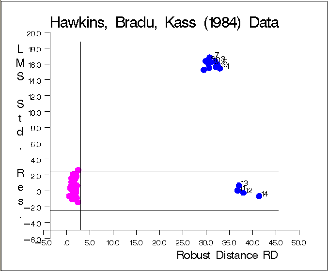
The graphs in Figure 9.6.5 and Figure 9.6.6 show the following:

the plot of standardized LMS residuals vs. robust distances
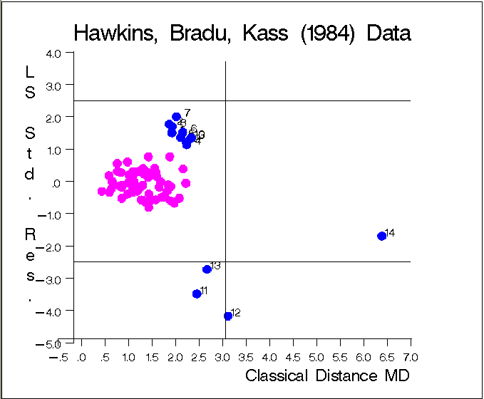
the plot of standardized LS residuals vs. Mahalanobis distances

The graph identifies the four good leverage points 11, 12, 13, and 14, which have small standardized LMS residuals but large robust distances, and the 10 bad leverage points

, which have large standardized LMS residuals and large robust distances.

Output 9.6.5: Hawkins-Bradu-Kass Data: LMS Residuals vs. Robust Distances

Output 9.6.6: Hawkins-Bradu-Kass Data: LS Residuals vs. Mahalanobis Distances

Top of Page