Language Reference: TSDECOMP Call :: SAS/IML(R) 9.2 User's Guide

Language Reference

TSDECOMP Call

analyzes nonstationary time series by using smoothness priors modeling

CALL TSDECOMP( comp, est, aic, data, <,xdata, order, sorder,

nar, npred, init, opt, icmp, print>);

The inputs to the TSDECOMP subroutine are as follows:

data

specifies a

(or

) data vector.

xdata

specifies a

explanatory data matrix.

order

specifies the order of trend differencing (0, 1, 2, or 3). The default is 2.

sorder

specifies the order of seasonal differencing (0, 1, or 2). The default is 1.

nar

specifies the order of the AR process. The default is 0.

npred

specifies the length of the forecast beyond the available observations. The default is 0.

init

specifies the initial values of parameters. The initial values are specified as variances for trend difference equation, AR process, seasonal difference equation, regression equation, and partial AR coefficients. The corresponding default variance values are 0.005, 0.8, 1E-5, and 1E-5. The default partial AR coefficient values are determined as

$\psi_i = 0.88 x (-0.6)^{i-1} \hspace*{.25in} i=1,2, ... ,{nar}$

opt

specifies the options vector.

opt[1]

specifies the mean deletion option. The mean of the original series is subtracted from the series if opt[1]=-1. By default, the original series is processed (opt[1]=0). When regressors are specified, only the opt[1]=0 option is accepted.

opt[2]

specifies the trading day adjustment. The default is opt[2]=0.

opt[3]

specifies the year ( $\geq 1900$ ) when the series starts. If opt[3]=0, there is no trading day adjustment. By default, opt[3]=0.

opt[4]

specifies the number of seasons within a period (speriod). By default, opt[4]=12.

opt[5]

controls the transformation of the original series. If opt[5]=1, log transformation is requested. By default, there is no transformation (opt[5]=0).

opt[6]

specifies the maximum number of iterations allowed. The default is opt[6] = 200.

opt[7]

specifies the update technique for the quasi-Newton optimization technique. If opt[7]=1 is specified, the dual Broyden, Fletcher, Goldfarb, and Shanno (BFGS) update method is used. If opt[7]=2 is specified, the dual Davidon, Fletcher, and Powell (DFP) update method is used. The default is opt[7]=1.

opt[8]

specifies the line search technique for the quasi-Newton optimization method. The default is opt[8] = 2.

opt[8]=1: specifies a line search method that requires the same number of objective function and gradient calls for cubic interpolation and extrapolation.
opt[8]=2: specifies a line search method that requires more objective function calls than gradient calls for cubic interpolation and extrapolation.
opt[8]=3: specifies a line search method that requires the same number of objective function and gradient calls for cubic interpolation and extrapolation.
opt[8]=4: specifies a line search method that requires the same number of objective function and gradient calls for cubic interpolation and stepwise extrapolation.
opt[8]=5: specifies a line search method that is a modified version of opt[8]=4.
opt[8]=6: specifies the golden section line search method that uses only function values for linear approximation.
opt[8]=7: specifies the bisection line search method that uses only function values for linear approximation.
opt[8]=8: specifies the Armijo line search method that uses only function values for linear approximation.

opt[9]

specifies the upper bound of the variance estimates. If you specify opt[9]=value, the variances are estimated with the constraint that $\sigma\leq {value}$ . When you specify the opt[9]=0 option, the upper bound is not imposed. The default is opt[9]=0.

opt[10]

specifies the length of data used in backward filtering for the Kalman filter initialization. The default value of opt[10] is 100 if the number of observations is greater than 100; otherwise, the default value is the number of observations.

icmp

specifies which component is calculated.

icmp=1: requests the estimate and forecast of trend component.
icmp=2: requests the estimate and forecast of seasonal component.
icmp=3: requests the estimate and forecast of AR component.
icmp=4: requests the trading day adjustment component.
icmp=5: requests the regression component.
icmp=6: requests the time-varying regression coefficients.

You can calculate multiple components by specifying a vector. For example, you can specify icmp={1 2 3 5}.

print

specifies the print option. By default, printed output is suppressed (print=0). If you specify print=1, the subroutine prints the final estimates. The iteration history is printed if you specify print=2.

The TSDECOMP subroutine returns the following values:

comp: refers to the estimate and forecast of the trend component.
est: refers to the parameter estimates including coefficients of the AR process.
aic: refers to the AIC statistic obtained from the final estimates.

The TSDECOMP subroutine analyzes nonstationary time series by using smoothness priors modeling (see the section "Smoothness Priors Modeling" for more details). The likelihood function is maximized with respect to hyperparameters. The Kalman filter algorithm is used for filtering, smoothing, and forecasting. The TSDECOMP call decomposes the time series $y_{t}$ as follows:

$y_t = t_t + s_t + t\!d_t + u_t + r_t + \epsilon_t$

where

represents the trend component,

denotes the seasonal component, $t\!d_t$ represents the trading day adjustment component,

denotes the autoregressive process component,

denotes regression effect components, and ${\epsilon}_t$ represents the irregular term with zero mean and constant variance.

The trend components are constrained as follows:

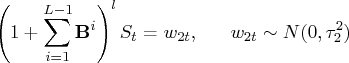
$\nabla^k t_t = w_{1t}, \hspace*{0.25in} w_{1t} \sim n(0,\tau_1^2)$

When you specify the ORDER=0 option, the trend component is not estimated. The maximum order of differencing is 3 (

).

The seasonal components are denoted as a stochastically perturbed equation:

$(1+\sum_{i=1}^{l-1} {b}^i)^l s_t = w_{2t}, \hspace*{0.25in} w_{2t} \sim n(0,\tau_2^2)$

When you specify SORDER=0, the seasonal component is not estimated. The maximum value of

is 2 (

).

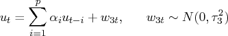
The stationary autoregressive (AR) process is denoted as a stochastically perturbed equation:

$u_t = \sum_{i=1}^p \alpha_i u_{t-i} + w_{3t}, \hspace*{0.25in} w_{3t} \sim n(0,\tau_3^2)$

where

is the order of AR process. When NAR=0 is specified, the AR process component is not estimated.

The time-varying regression coefficients are estimated if you include exogenous variables:

$r_t = {x}_t\beta_t$

where ${x}_t$ contains

regressors except the constant term and $\beta^'_t = (\beta_{1t}, ... ,\beta_{mt})$ . The time-varying coefficients $\beta_t$ follow the random walk process:

$\beta_{jt} = \beta_{jt-1} + v_{jt}, \hspace*{0.25in} v_{jt} \sim n(0,\sigma_j^2)$

where $\beta_{jt}$ is an element of the coefficient vector $\beta_t$ .

The trading day adjustment component $t\!d_t$ is deterministically restricted. See the section "State Space and Kalman Filter Method", for more information.

You can estimate the time-varying coefficient model as follows:

  
    call tsdecomp COMP=beta ORDER=0 SORDER=0 NAR=0 
                  DATA=y XDATA=x ICMP=6;

The output matrix BETA contains time-varying regression coefficients.

Top of Page