Language Reference: TPSPLINE Call :: SAS/IML(R) 9.2 User's Guide

Language Reference

TPSPLINE Call

computes thin-plate smoothing splines

CALL TPSPLINE( fitted, coeff, adiag, gcv, , $y\lt$ , lambda> );

The TSPLINE subroutine computes thin-plate smoothing spline (TPSS) fits to approximate smooth multivariate functions that are observed with noise. The generalized cross validation (GCV) function is used to select the smoothing parameter.

The TPSPLINE subroutine returns the following values:

fitted: is an vector of fitted values of the TPSS fit evaluated at the design points . The is the number of observations. The final TPSS fit depends on the optional lambda.
coeff: is a vector of spline coefficients. The vector contains the coefficients for basis functions in the null space and the representer of evaluation functions at unique design points. (Refer to Wahba 1990 for more detail on reproducing kernel Hilbert space and representer of evaluation functions.) The length of coeff vector depends on the number of unique design points and the number of variables in the spline model. In general, let nuobs and be the number of unique rows and the number of columns of respectively. The length of coeff equals to . The coeff vector can be used as an input of TPSPLNEV to evaluate the resulting TPSS fit at new data points.
adiag: is an vector of diagonal elements of the "hat" matrix. See the "Details" section.
gcv: If lambda is not specified, then gcv is the minimum value of the GCV function. If lambda is specified, then gcv is a vector (or scalar if lambda is a scalar) of GCV values evaluated at the lambda points. It provides you with both the ability to study the GCV curves by plotting gcv against lambda and the chance to identify a possible local minimum.

The inputs to the TPSPLINE subroutine are as follows:

: is an matrix of design points on which the TPSS is to be fit. The is the number of variables in the spline model. The columns of need to be linearly independent and contain no constant column.
: is the vector of observations.
lambda: is a optional vector containing $\lambda$ values in $log_{10}(n\lambda)$ scale. This option gives you the power to control how you want the TPSPLINE subroutine to function. If lambda is not specified (or lambda is specified and $q \gt 1$ ) the GCV function is used to choose the "best" $\lambda$ and the returning fitted values are based on the $\lambda$ that minimizes the GCV function. If lambda is specified and , no minimization of the GCV function is involved and the fitted, coeff and adiag values are all based on the TPSS fit using this particular lambda. This gives you the freedom to choose the $\lambda$ that you deem appropriate.

Aside from the values returned, the TPSPLINE subroutine also prints other useful information such as the number of unique observations, the dimensions of the null space, the number of parameters in the model, a GCV estimate of $\lambda$ , the smoothing penalty, the residual sum of square, the trace of $(i-a(\lambda))$ , an estimate of $\sigma^2$ , and the sum of squares for replication.

Note: No missing values are accepted within the input arguments. Also, you should use caution if you want to specify small lambda values. Since the true $\lambda=(10^{\log_{10} {lambda}})/n$ , a very small value for lambda can cause $\lambda$ to be smaller than the magnitude of machine error and usually the returned gcv values from such a $\lambda$ cannot be trusted. Finally, when using TPSPLINE be aware that TPSS is a computationally intensive method. Therefore a large data set (that is, a large number of unique design points) will take a lot of computer memory and time.

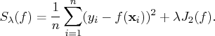
For convenience, the TPSS method is illustrated with a two-dimensional independent variable ${x}=({x}^1,{x}^2)$ . More details can be found in Wahba (1990), or in Bates et al. (1987).

Assume that the data are from the model

$y_i = f({{x}}_i) + \epsilon_i,$

where $({{x}}_i, y_i), i=1, ... ,n$ are the observations. The function

is unknown and you assume that it is reasonably smooth. The error terms $\epsilon_i, i=1, ... ,n$ are independent zero-mean random variables.

You measure the smoothness of

by the integral over the entire plane of the square of the partial derivatives of

of total order 2, that is

$j_2(f) = \int_{-\infty}^{\infty} \int_{-\infty}^{\infty} [ \frac{\partial^2 f}... ...rtial {x_2}} ]^2 + [ \frac{\partial^2 f}{\partial {x_2}^2} ]^2 dx_1 dx_2$

Using this as a smoothness penalty, the thin-plate smoothing spline estimate $f_{\lambda}$ of

is the minimizer of

$s_\lambda(f) = \frac{1}n \sum^n_{i=1} (y_i-f({x}_i))^2 + \lambda j_2(f).$

Duchon (1976) derived that the minimizer $f_{\lambda}$ can be represented as

$f_\lambda({x}) = \sum_{i=1}^3 \beta_i \phi_i({x}) + \sum_{i=1}^n \delta_i e_2({x}-{x}_i),$

where $(\phi_1({x}),\phi_2({x}),\phi_3({x})) = (1,{x}^1,{x}^2)$ and $e_2(\bs)=\frac{1}{2^3 \pi} \vert\bs\vert^2ln(\vert\bs\vert)$ .

Let matrix

have entries $({k})_{ij} = e_2({x}_i-{x}_j)$ and matrix

have entries $({t})_{ij} = \phi_j({x}_i)$ . Then the minimization problem can be rewritten as finding coefficients $\beta$ and $\delta$ to minimize

$s_\lambda(\beta, \delta) = \frac{1}n \vert {y}- {t}\beta - {k}\delta \vert^2 + \lambda \delta^t {k}\delta$

The final TPSS fits can be viewed as a type of generalized ridge regression estimator. The $\lambda$ is called the smoothing parameter, which controls the balance between the goodness of fit and the smoothness of the final estimate. The smoothing parameter can be chosen by minimizing the generalized cross validation function (GCV). If you write

$\hat{{y}} = {a}(\lambda) {y}$

and call the ${a}(\lambda)$ as the ``

'' matrix, the GCV function $v(\lambda)$ is defined as

$v(\lambda) = \frac{(1/n) \vert({i}- {a}(\lambda) {y}\vert^2} {[(1/n) {tr}({i}- {a}(\lambda))]^2}$

The returned values from this function call provide the $\hat{{y}}$ as fitted, the $(\beta,\delta)$ as coeff, and $diag(a(\lambda))$ as adiag.

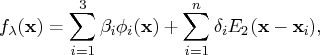
To evaluate the TPSS fit $f_\lambda({x})$ at new data points, you can use the TPSPLNEV call.

Suppose ${x}^{new}$ , a

matrix, contains the

new data points at which you want to evaluate $f_{\lambda}$ . Let $({t}^{new}_{ij}) = \phi_j({x}^{new}_i)$ and $({k}^{new}_{ij})=e_2({x}^{new}_i-{x}_j)$ be the

th elements of ${t}^{new}$ and ${k}^{new}$ respectively. The prediction at new data points ${x}^{new}$ is

${y}_{pred}=t^{new} \beta + k^{new} \delta$

Therefore, using the coefficient $(\beta,\delta)$ obtained from TPSPLINE call, the ${y}_{pred}$ can be easily evaluated.

An example is given in the documentation for the TPSPLNEV call.

Top of Page