Language Reference

TPSPLNEV Call

evaluates the thin-plate smoothing spline at new data points

It can be used only after the TPSPLINE call.

CALL TPSPLNEV( pred, xpred, , coeff);

The TPSPLNEV subroutine returns the following value:

pred

is an vector of the predicated values of the TPSS fit evaluated at new data points.

The inputs to the TPSPLNEV subroutine are as follows:

xpred

is an matrix of data points at which the is evaluated, where is the number of new data points and is the number of variables in the spline model.

is an matrix of design points that is used as an input of TPSPLINE call.

coeff

is the coefficient vector returned from the TPSPLINE call.

See the previous section on the TPSPLINE call for details about the TSPLNEV subroutine.

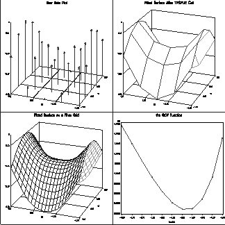
As an example, consider the following data set, which consists of two independent variables. The plot of the raw data can be found in the first panel of Figure 20.1.

  
    x={ -1.0 -1.0,    -1.0 -1.0,     -.5 -1.0,     -.5 -1.0, 
          .0 -1.0,      .0 -1.0,      .5 -1.0,      .5 -1.0, 
         1.0 -1.0,     1.0 -1.0,     -1.0 -.5,     -1.0 -.5, 
          -.5 -.5,      -.5 -.5,       .0 -.5,       .0 -.5, 
           .5 -.5,       .5 -.5,      1.0 -.5,      1.0 -.5, 
          -1.0 .0,      -1.0 .0,       -.5 .0,       -.5 .0, 
            .0 .0,        .0 .0,        .5 .0,        .5 .0, 
           1.0 .0,       1.0 .0,      -1.0 .5,      -1.0 .5, 
           -.5 .5,       -.5 .5,        .0 .5,        .0 .5, 
            .5 .5,        .5 .5,       1.0 .5,       1.0 .5, 
         -1.0 1.0,     -1.0 1.0,      -.5 1.0,      -.5 1.0, 
           .0 1.0,       .0 1.0,       .5 1.0,       .5 1.0, 
          1.0 1.0,      1.0 1.0 }; 
  
    y={15.54483570,  15.76312613,   18.67397826,   18.49722167, 
       19.66086310,  19.80231311,   18.59838649,   18.51904737, 
       15.86842815,  16.03913832,   10.92383867,   11.14066546, 
       14.81392847,  14.82830425,   16.56449698,   16.44307297, 
       14.90792284,  15.05653924,   10.91956264,   10.94227538, 
       9.614920104,  9.646480938,   14.03133439,   14.03122345, 
       15.77400253,  16.00412514,   13.99627680,   14.02826553, 
       9.557001644,  9.584670472,   11.20625177,   11.08651907, 
       14.83723493,  14.99369172,   16.55494349,   16.51294369, 
       14.98448603,  14.71816070,   11.14575565,   11.17168689, 
       15.82595514,  15.96022497,   18.64014953,   18.56095997, 
       19.54375504,  19.80902641,   18.56884576,   18.61010439, 
       15.86586951,  15.90136745 };
 

Now generate a sequence of from -3.8 to -3.3 so that you can study the GCV function within this range. Use the following statement:

  
    lambda=T(do(-3.8,-3.3,0.1));
 

Use the following IML statement to do the thin-plate smoothing spline fit and returning the fitted values on those design points.

  
    call tpspline(fit,coef,adiag,gcv, x, y,lambda);
 

The output from this call follows.

  
                    SUMMARY OF TPSPLINE CALL 
  
         Number of observations                    50 
         Number of unique design points            25 
         Dimension of polynomial Space              3 
         Number of Parameters                      28 
  
  
  
         GCV Estimate of Lambda              0.00000668 
         Smoothing Penalty                   2558.14323 
         Residual Sum of Squares                0.24611 
         Trace of (I-A)                        25.40680 
         Sigma^2 estimate                       0.00969 
         Sum of Squares for Replication         0.24223
 

After this TPSPLINE call, you obtained the fitted value. The fitted surface is plotted in the second panel of Figure 20.1. Also in Figure 20.1, panel 4, you plot the GCV function values against lambda. From panel 2, you see that because of the spare design points, the fitted surface is a little bit rough. In order to study the TPSS fit more closely, you use the following IML statements to generate a more dense grid on .

  
    do i1=-1 to 1 by 0.1; 
       do i2=-1 to 1 by 0.1; 
          x1=x1||i1; 
          x2=x2||i2; 
       end; 
    end; 
    x1=t(x1); 
    x2=t(x2); 
    xpred=x1||x2;
 

Now you can use the function TPSPLNEV to evaluate on this dense grid. Here is the statement:

  
    call tpsplnev(pred,  xpred, x, coef);
 

The final fitted surface is plotted in Figure 20.1, panel 3.

Figure 20.1: Plots of Fitted Surface