Managing the Graphical Output

Directing Output to ODS Destinations

All ODS graphics are generated in industry standard formats (PNG, PDF, and so on), depending on the settings for the active ODS destinations. The ODS HTML destination is on by default, and the default image format for the HTML destination is PNG.

All ODS destinations such as HTML, PDF, RTF, LATEX, and PRINTER are fully supported. The ODS destinations enable you to

manage the graphs that are generated by ODS Graphics
display the output in a variety of forms (HTML, PDF, RTF, ...)
control the location of stored output files and other features that are relevant for the active destinations.

As discussed in Compiling the Template, a compiled template is stored in an item store. Thus, without rewriting or resubmitting the template code, we can render the graph as often as needed during the current SAS session or a future SAS session.

To generate ODS Graphics output for use on the Web, we can direct the output to the HTML destination, which generates an image file for the graph, and also an HTML file that references the image. Thus, output that is generated in the HTML destination is ready for display in a Web browser.

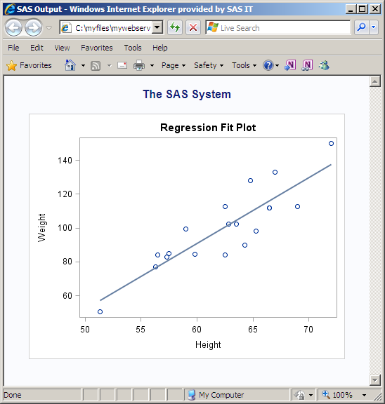
The following ODS HTML statement stores the output files in the folder C:\myfiles\mywebserver. The code first closes the LISTING destination to avoid creating extra output:

ods html path="C:\myfiles\mywebserver" (url=none) file="modelfit.html" ;
proc sgrender data=sashelp.class template=modelfit; run;
ods html close; /* to close the output file */
ods listing; /* reopen the HTML destination for subsequent output */

The PATH= option specifies storage location C:\myfiles\mywebserver for output files that are created by the SAS statements, including images from ODS Graphics.
The FILE= option specifies that SAS output is written to the file modelfit.html, which is saved in the location specified on PATH=.
The ODS HTML CLOSE statement closes the HTML destination, which enables you to see your output. By default, the HTML destination uses the HTMLBLUE style for graphics output (Modifying Graph Appearance with Styles provides an introduction to ODS styles), which uses a gray background.

Regression Fit Plot Directed to HTML Destination

See Managing Graphical Output for more information about the ODS destinations and the type of output that results from each destination.

Modifying Graph Appearance with Styles

GTL has been designed to be totally integrated with ODS styles.

Note: Although every appearance detail of a graph is controlled by the current style by default, you can use GTL syntax options to change the appearance of the graph.

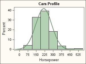
The following template code generates the histogram that was introduced in Defining the Graph Template.

proc template;
  define statgraph cars;
    begingraph;
      entrytitle "Cars Profile";
      layout overlay;
        histogram horsepower;
        densityplot horsepower;
      endlayout;
    endgraph;
  end;
run;

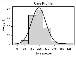
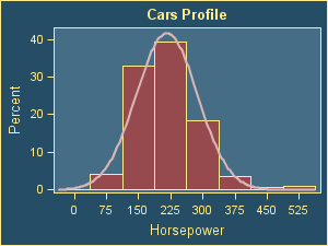
Every ODS destination has a style that it uses by default. For the HTML destination, the default style is HTMLBlue. To modify the appearance of the graph, you can change its style by specifying the STYLE= option in the ODS destination statement before running the SGRENDER procedure:

ods html style=analysis ;
proc sgrender data=sashelp.cars template=cars;
run;

ods html style=journal ;
proc sgrender data=sashelp.cars template=cars;
run;

ods html style=astronomy ;
proc sgrender data=sashelp.cars template=cars;
run;

For more information about how the appearance of the graph is determined and the ways that you can modify it, see Managing Graph Appearance: General Principles and Managing the Graph Appearance with Styles.

Controlling Physical Aspects of the Output

The ODS GRAPHICS statement provides options that control the physical aspects of your graphs, such as the graph size and the name of the output image file.

The HTML destination's default image size of 640 pixels by 480 pixels (4:3 aspect ratio) for ODS Graphics is set in the SAS Registry. You can change the graph size using the ODS GRAPHICS statement’s WIDTH= and/or HEIGHT= options. To name the output image file, use the IMAGENAME= option.

The following ODS GRAPHICS statement sets a 320 pixel width for the graph and names the output image modelfitgraph:

ods graphics / width=320px imagename=”modelfitgraph” ;

proc sgrender data=sashelp.class template=modelfit;
run;

ods graphics / reset ;

The WIDTH= option sets the image width to 320 pixels. Because no HEIGHT= option is used, SAS uses the design aspect ratio of the graph to compute the appropriate height. (The width of 320px is half the default width, so SAS will set the height to 240px, which is half the default height.) In general, it is good practice to specify only one sizing option without the other — just the WIDTH= option or just the HEIGHT= option. That way SAS will maintain the design aspect ratio of the graph, which might be important for many graphs.
The IMAGENAME= option in the first ODS GRAPHICS statement sets the name of the output image file to modelfitgraph.
The RESET option in the second ODS GRAPHICS statement resets all ODS GRAPHICS options to their default state. If the options are not reset, all subsequent graphs would be 320 pixels wide and image names would be assigned incremental names (modelfitgraph1, modelfitgraph2, and so on) every time a graph is produced.

For more information about the details of managing image name, image size, image format, and DPI., see Managing Graphical Output.