The EM Algorithm

The EM algorithm (Excoffier and Slatkin 1995; Hawley and Kidd 1995; Long, Williams, and Urbanek 1995) iteratively furnishes the maximum likelihood estimates (MLEs) of -locus haplotype frequencies, for any integer , when a direct solution for the MLE is not readily feasible. The EM algorithm assumes HWE; it has been argued (Fallin and Schork 2000) that positive increases in the Hardy-Weinberg disequilibrium coefficient (toward excess heterozygosity) can increase the error of the EM estimates, but negative increases (toward excess homozygosity) do not demonstrate a similar increase in the error. The iterations start with assigning initial values to the haplotype frequencies. When the INIT=RANDOM option is included in the PROC HAPLOTYPE statement, uniformly distributed random values are assigned to all haplotype frequencies; when INIT=UNIFORM, each haplotype is given an initial frequency of , where is the number of possible haplotypes in the sample. Otherwise, the product of the frequencies of the alleles that constitute the haplotype is used as the initial frequency for the haplotype. Different starting values can lead to different solutions since a maximum that is found could be a local maximum and not the global maximum. You can try different starting values for the EM algorithm by specifying a number greater than 1 in the NSTART= option to get better estimates. The expectation and maximization steps (E step and M step, respectively) are then carried out until the convergence criterion is met or the number of iterations exceeds the number specified in the MAXITER= option of the PROC HAPLOTYPE statement.

For a sample of individuals, suppose the th individual has genotype . The probability of this genotype in the population is , so the log likelihood is

which is calculated after each iteration’s E step of the EM algorithm, described in the following paragraphs.

Let be the th possible haplotype, and let be its frequency in the population. For genotype , the set is the collection of pairs of haplotypes, and its "complement" , that constitute that genotype. The haplotype frequencies used in the E step for iteration 0 of the EM algorithm are given by the initial values; all subsequent iterations use the haplotype frequencies calculated by the M step of the previous iteration. The E step sets the genotype frequencies to be products of these frequencies:

When has heterozygous loci, there are terms in this sum. The number of times haplotype occurs in the sum is written as , which is 2 if is completely homozygous, and either 1 or 0 otherwise.

The M step sets new haplotype frequencies from the genotype frequencies:

The EM algorithm increases the likelihood after each iteration, and multiple starting points can generally lead to the global maximum.

When the option EST=STEPEM is specified in the PROC HAPLOTYPE statement, a stepwise version of the EM algorithm is performed. A common difficulty in haplotype analysis is that the number of possible haplotypes grows exponentially with the number of loci, as does the computation time, which makes the EM algorithm infeasible for a large number of loci. However, the most common haplotypes can still be estimated by trimming the haplotype table according to a given cutoff (Clayton 2002). The two-locus haplotype frequencies are first estimated, and those below the cutoff are discarded from the table. The remaining haplotypes are expanded to the next locus by forming all possible three-locus haplotypes, and the EM algorithm is then invoked for this haplotype table. The trimming and expanding process is performed repeatedly, adding one locus at a time, until all loci are considered.

After the EM or stepwise EM algorithm has arrived at the MLEs of the haplotype frequencies, each individual ’s probability of having a particular haplotype pair given the individual’s genotype is calculated as

for each . These probabilities are displayed in the OUT= data set.

Methods of Estimating Standard Error

Typically, an estimate of the variance of a haplotype frequency is obtained by inverting the estimated information matrix from the distribution of genotype frequencies. However, it often turns out that in a large multilocus system, a certain proportion of haplotypes have ML frequencies equal or close to zero, which makes the sample information matrix nearly singular (Excoffier and Slatkin 1995). Therefore, two approximation methods are used to estimate the variances, as proposed by Hawley and Kidd (1995).

The binomial method estimates the standard error by calculating the square root of the binomial variance, as if the haplotype frequencies are obtained by direct counting:

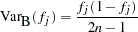The jackknife method is a simulation-based method that can be used to estimate the standard errors of haplotype frequencies. Each individual is in turn removed from the sample, and all the haplotype frequencies are recalculated from this "delete-1" sample. Let be the haplotype frequency estimator from the th "delete-1" sample; then the jackknife variance estimator has the following formula:

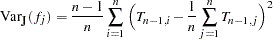and the square root of this variance estimate is the estimate of standard error. The jackknife is less dependent on the model assumptions; however, it requires computing the statistic times.

Confidence intervals with confidence level for the haplotype frequency estimates from the final iteration are then calculated using the following formula:

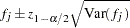where is the value from the standard normal distribution that has a right-tail probability of .

Testing for Allelic Associations

When the LD option is specified in the PROC HAPLOTYPE statement, haplotype frequencies are calculated using the EM algorithm as well as by assuming no allelic associations among loci—that is, no LD. Under the null hypothesis of no LD, haplotype frequencies are simply the product of the individual allele frequencies. The log likelihood under the null hypothesis, , is calculated based on these haplotype frequencies with degrees of freedom 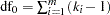, where is the number of loci and is the number of alleles for the th locus (Zhao, Curtis, and Sham 2000). Under the alternative hypothesis, the log likelihood, , is calculated from the EM estimates of the haplotype frequencies with degrees of freedom . A likelihood ratio test is used to test this hypothesis as follows:

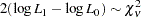where is the difference between the number of degrees of freedom under the null hypothesis and the alternative.

Testing for Trait Associations

When the TRAIT statement is included in PROC HAPLOTYPE, case-control tests are performed to test for association between the dichotomous trait (often, an indicator of individuals with or without a disease) and the marker loci by using haplotypes. In addition to an omnibus test that is performed across all haplotypes, when the TESTALL option is specified in the TRAIT statement, a test for association between each individual haplotype and the trait is performed. Note that the individual haplotype tests should be performed only if the omnibus test statistic is significant.

Chi-Square Tests

The test performed over all haplotypes is based on the log likelihoods: under the null hypothesis, the log likelihood over all the individuals in the sample, regardless of the value of their trait variable, is calculated as described in The EM Algorithm; the log likelihood is also calculated separately for the two sets of individuals within the sample as determined by the trait value under the alternative hypothesis of marker-trait association. A likelihood ratio test (LRT) statistic can then be formed as follows:

where , , and are the log likelihoods under the null hypothesis, for individuals with the first trait value, and for individuals with the second trait value, respectively (Zhao, Curtis, and Sham 2000). Defining degrees of freedom for each log likelihood similarly, this statistic has an asymptotic chi-square distribution with degrees of freedom.

An association between individual haplotypes and the trait can also be tested. To do so, a contingency table (Table 8.1) is formed where , the total number of haplotypes in the sample, "Hap 1" refers to the current haplotype being tested, "Hap 2" refers to all other haplotypes, and is the pseudo-observed count of individuals with trait and haplotype (note that these counts are not necessarily integers since haplotypes are not actually observed; they are calculated based on the estimated haplotype frequencies). The column totals are not calculated in the usual fashion, by summing the cells in each column; rather, and are calculated as and , respectively, where is the estimated frequency of "Hap 1" in the overall sample.

Table 8.1 Haplotype-Trait Counts

	Hap 1	Hap 2	Total
Trait 1
Trait 2
Total

The usual contingency table chi-square test statistic has a 1 df chi-square distribution:

Permutation Tests

Since the assumption of a chi-square distribution in the preceding section might not hold, estimates of exact -values via Monte Carlo methods are recommended. New samples are formed by randomly permuting the trait values, and either of the chi-square test statistics shown in the previous section can be calculated for each of these samples. The number of new samples created is determined by the number given in the PERMS= option of the TRAIT statement. The exact -value approximation is then calculated as , where is the number of samples with a test statistic greater than or equal to the test statistic in the actual sample and is the total number of permutation samples. This method is used to obtain empirical -values for both the overall and the individual haplotype tests (Zhao, Curtis, and Sham 2000; Fallin et al. 2001).

Bayesian Estimation of Haplotype Frequencies

The Bayesian algorithm for haplotype reconstruction incorporates coalescent theory in a Markov chain Monte Carlo (MCMC) technique (Stephens, Smith, and Donnelly 2001; Lin et al. 2002). The algorithm starts with a random phase assignment for each multilocus genotype and then uses a Gibbs sampler to assign a haplotype pair to a randomly picked phase-unknown genotype. The algorithm implemented in PROC HAPLOTYPE is from Lin et al. (2002), which has several variations from that of Stephens, Smith, and Donnelly (2001).

Initially, gamete pairs are randomly assigned to each genotype, and the assignment set is denoted as . An individual is then randomly picked, and its two current haplotypes are removed from . The remaining assignment set is denoted . Let be the positions where the diplotypic sequence of individual is ambiguous, and let be the partial sequence of the th haplotype at . From , a list of partial haplotypes is made, with corresponding counts sampled from .

The next step is to reassign a haplotype pair to individual and add to . The probability vector, , of sampling each partial haplotype from is calculated as follows: let be the partial genotype of individual at . For , check whether can comprise plus a complementary haplotype (note that can bear missing alleles if is incomplete). If not, set ; if so, with all in that are compatible with , set , where by default (or this value can be set in the THETA= option), is the number of individuals in the sample, and is the number of distinct haplotypes possible in the population. If no such can be found, set .

With probability , being the number of ambiguous sites in individual , randomly reconstruct phases for individual . Missing alleles are assigned proportional to allele frequencies at each site. Otherwise, with probability , assign to individual and the corresponding complementary haplotype. The new assignment is then added back to .

These steps are repeated times, where is the value specified in the TOTALRUN= option. The first times are discarded as burn-in when BURNIN=. The results are then thinned by recording every th assignment specified by the INTERVAL= option so that iterations are used for the estimates.

The probability of each individual having a particular haplotype pair given the individual’s genotype for each is given in the OUT= data set as the proportion of iterations after burn-in that are recorded which have that particular haplotype pair assigned to the individual.