The AUTOREG Procedure
- Overview
-
Getting Started

-
Syntax
-
DetailsMissing ValuesAutoregressive Error ModelAlternative Autocorrelation Correction MethodsGARCH ModelsHeteroscedasticity- and Autocorrelation-Consistent Covariance Matrix EstimatorGoodness-of-Fit Measures and Information CriteriaTestingPredicted ValuesOUT= Data SetOUTEST= Data SetPrinted OutputODS Table NamesODS Graphics
-
Examples
- References
Heteroscedasticity- and Autocorrelation-Consistent Covariance Matrix Estimator
The heteroscedasticity-consistent covariance matrix estimator (HCCME), also known as the sandwich (or robust or empirical) covariance matrix estimator, has been popular in recent years because it gives the consistent estimation of the covariance matrix of the parameter estimates even when the heteroscedasticity structure might be unknown or misspecified. White (1980) proposes the concept of HCCME, known as HC0. However, the small-sample performance of HC0 is not good in some cases. Davidson and MacKinnon (1993) introduce more improvements to HC0, namely HC1, HC2 and HC3, with the degrees-of-freedom or leverage adjustment. Cribari-Neto (2004) proposes HC4 for cases that have points of high leverage.
HCCME can be expressed in the following general "sandwich" form:
![\[ \Sigma =B^{-1} M B^{-1} \]](images/etsug_autoreg0317.png)
where B, which stands for "bread," is the Hessian matrix and M, which stands for "meat," is the outer product of gradient (OPG) with or without adjustment. For HC0, M is the OPG without adjustment; that is,
![\[ M_{\mr{HC0}}=\sum _{t=1}^{T}{g_ t g_ t’} \]](images/etsug_autoreg0318.png)
where T is the sample size and  is the gradient vector of tth observation. For HC1, M is the OPG with the degrees-of-freedom correction; that is,
![\[ M_{\mr{HC1}}=\frac{T}{T-k}\sum _{t=1}^{T}{g_ t g_ t’} \]](images/etsug_autoreg0320.png)
where k is the number of parameters. For HC2, HC3, and HC4, the adjustment is related to leverage, namely,
![\[ M_{\mr{HC2}}=\sum _{t=1}^{T}{\frac{g_ t g_ t'}{1-h_{tt}}} \\ M_{\mr{HC3}}=\sum _{t=1}^{T}{\frac{g_ t g_ t'}{(1-h_{tt})^2}} \\ M_{\mr{HC4}}=\sum _{t=1}^{T}{\frac{g_ t g_ t'}{(1-h_{tt})^{\min {(4,T h_{tt}/k)}}}} \]](images/etsug_autoreg0321.png)
The leverage  is defined as
 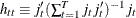 , where
  is defined as follows:
-
For an OLS model,
is the tth observed regressors in column vector form.
-
For an AR error model,
is the derivative vector of the tth residual with respect to the parameters.
-
For a GARCH or heteroscedasticity model,
is the gradient of the tth observation (that is, ).
The heteroscedasticity- and autocorrelation-consistent (HAC) covariance matrix estimator can also be expressed in "sandwich" form:
where B is still the Hessian matrix, but M is the kernel estimator in the following form:
![\[ M_{\mr{HAC}}=a\left(\sum _{t=1}^{T}{g_ t g_ t’}+\sum _{j=1}^{T-1}{k\left(\frac{j}{b}\right)\sum _{t=1}^{T-j}{\left(g_ t g_{t+j}’ + g_{t+j} g_{t}’\right)}}\right) \]](images/etsug_autoreg0325.png)
where T is the sample size, is the gradient vector of tth observation,  is the real-valued kernel function, b is the bandwidth parameter, and a is the adjustment factor of small-sample degrees of freedom (that is,
  if ADJUSTDF option is not specified and otherwise
  , where k is the number of parameters). The types of kernel functions are listed in Table 9.2.
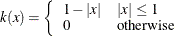
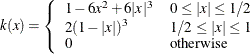
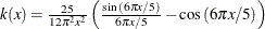
Table 9.2: Kernel Functions
|
Kernel Name |
Equation |
|---|---|
|
Bartlett |
|
|
Parzen |
|
|
Quadratic spectral |
|
|
Truncated |
|
|
Tukey-Hanning |
|
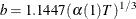
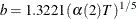
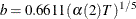
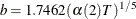
When you specify BANDWIDTH=ANDREWS91, according to Andrews (1991) the bandwidth parameter is estimated as shown in Table 9.3.
Table 9.3: Bandwidth Parameter Estimation
|
Kernel Name |
Bandwidth Parameter |
|---|---|
|
Bartlett |
|
|
Parzen |
|
|
Quadratic spectral |
|
|
Truncated |
|
|
Tukey-Hanning |
|
Let  denote each series in
  , and let
  denote the corresponding estimates of the autoregressive and innovation variance parameters of the AR(1) model on ,
  , where the AR(1) model is parameterized as
 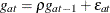 with
with  . The factors
  and
and  are estimated with the following formulas:
![\[ \alpha (1) = \frac{\sum _{a=1}^ k{\frac{4\rho _ a^2\sigma _ a^4}{(1-\rho _ a)^6(1+\rho _ a)^2}}}{\sum _{a=1}^ k{\frac{\sigma _ a^4}{(1-\rho _ a)^4}}} \\ \alpha (2) = \frac{\sum _{a=1}^ k{\frac{4\rho _ a^2\sigma _ a^4}{(1-\rho _ a)^8}}}{\sum _{a=1}^ k{\frac{\sigma _ a^4}{(1-\rho _ a)^4}}} \]](images/etsug_autoreg0347.png)
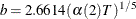
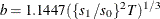
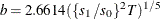
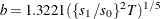
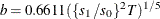
When you specify BANDWIDTH=NEWEYWEST94, according to Newey and West (1994) the bandwidth parameter is estimated as shown in Table 9.4.
Table 9.4: Bandwidth Parameter Estimation
|
Kernel Name |
Bandwidth Parameter |
|---|---|
|
Bartlett |
|
|
Parzen |
|
|
Quadratic spectral |
|
|
Truncated |
|
|
Tukey-Hanning |
|
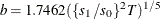
The factors  and
and  are estimated with the following formulas:
![\[ s_1 = 2\sum _{j=1}^ n{j\sigma _ j} \\ s_0 = \sigma _0+2\sum _{j=1}^ n{\sigma _ j} \]](images/etsug_autoreg0355.png)
where n is the lag selection parameter and is determined by kernels, as listed in Table 9.5.
Table 9.5: Lag Selection Parameter Estimation
|
Kernel Name |
Lag Selection Parameter |
|---|---|
|
Bartlett |
|
|
Parzen |
|
|
Quadratic spectral |
|
|
Truncated |
|
|
Tukey-Hanning |
|
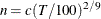
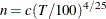
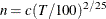
The factor c in Table 9.5 is specified by the C= option; by default it is 12.
The factor  is estimated with the equation
![\[ \sigma _ j = T^{-1}\sum _{t=j+1}^{T}{\left(\sum _{a=i}^ k{g_{at}}\sum _{a=i}^ k{g_{at-j}}\right)}, j=0, ..., n \]](images/etsug_autoreg0361.png)
where i is 1 if the NOINT option in the MODEL statement is specified (otherwise, it is 2), and  is the same as in the Andrews method.
If you specify BANDWIDTH=SAMPLESIZE, the bandwidth parameter is estimated with the equation
![\[ b = \left\{ \begin{array}{ l l } \left\lfloor {\gamma T^{r} + c} \right\rfloor & \text {if BANDWIDTH=SAMPLESIZE(INT) option is specified} \\ \gamma T^{r} + c & \text {otherwise} \end{array} \right. \]](images/etsug_autoreg0363.png)
where T is the sample size;  is the largest integer less than or equal to x; and
  , r, and c are values specified by the BANDWIDTH=SAMPLESIZE(GAMMA=, RATE=, CONSTANT=) options, respectively.
If you specify the PREWHITENING option, is prewhitened by the VAR(1) model,
![\[ g_ t = A g_{t-1} + w_ t \]](images/etsug_autoreg0365.png)
Then M is calculated by
![\[ M_{\mr{HAC}}=a(I-A)^{-1}\left(\sum _{t=1}^{T}{w_ t w_ t’} +\sum _{j=1}^{T-1}{k\left(\frac{j}{b}\right) \sum _{t=1}^{T-j}{\left(w_ t w_{t+j}’ + w_{t+j} w_{t}’\right)}}\right)\left((I-A)^{-1}\right)’ \]](images/etsug_autoreg0366.png)
The bandwidth calculation is also based on the prewhitened series  .
.