The COUNTREG Procedure
- Overview
- Getting Started
-
Syntax

-
DetailsSpecification of RegressorsMissing ValuesPoisson RegressionConway-Maxwell-Poisson RegressionNegative Binomial RegressionZero-Inflated Count Regression OverviewZero-Inflated Poisson RegressionZero-Inflated Conway-Maxwell-Poisson RegressionZero-Inflated Negative Binomial RegressionVariable SelectionPanel Data AnalysisComputational ResourcesNonlinear Optimization OptionsCovariance Matrix TypesDisplayed OutputOUTPUT OUT= Data SetOUTEST= Data SetODS Table NamesODS Graphics
-
Examples
- References
This type of variable selection uses either Akaike’s information criterion (AIC) or the Schwartz Bayesian criterion (SBC) and either a forward selection method or a backward elimination method.
Forward selection starts from a small subset of variables. In each step, the variable that gives the largest decrease in the value of the information criterion specified in the CRITER= option (AIC or SBC) is added. The process stops when the next candidate to be added does not reduce the value of the information criterion by more than the amount specified in the LSTOP= option in the MODEL statement.
Backward elimination starts from a larger subset of variables. In each step, one variable is dropped based on the information criterion chosen.
You can force a variable to be retained in the variable selection process by adding a RETAIN list to the SELECT=INFO (or SELECTVAR=) option in your model. For example, suppose you add a RETAIN list to the SELECT=INFO option in your model as follows:
MODEL Art = Mar Kid5 Phd / dist=negbin(p=2) SELECT=INFO(lstop=0.001 RETAIN(Phd));
Then this causes the variable selection process to consider only those models that contain Phd as a regressor. As a result, you are guaranteed that Phd will appear as one of the regressor variables in whatever model the variable selection process produces. The model that results
is the “best” (relative to your selection criterion) of all the possible models that contain Phd.
When a ZEROMODEL statement is used in conjunction with a MODEL statement, then all the variables that appear in the ZEROMODEL statement are retained by default unless the ZEROMODEL statement itself contains a SELECT=INFO option.
For example, suppose you have the following:
   MODEL Art = Mar Kid5 Phd  / dist=negbin(p=2) SELECT=INFO(lstop=0.001 RETAIN(Phd));
   ZEROMODEL Art ~ Fem Ment / link=normal;
Then Phd is retained in the MODEL statement and all the variables in the ZEROMODEL statement (Fem and Ment) are retained as well. You can add an empty SELECT=INFO clause to the ZEROMODEL statement to indicate that all the variables
in that statement are eligible for elimination (that is, need not be retained) during variable selection. For example:
  MODEL Art = Mar Kid5 Phd  / dist=negbin(p=2) SELECT=INFO(lstop=0.001 RETAIN(Phd));
  ZEROMODEL Art ~ Fem Ment / link=normal SELECT=INFO();
In this example, only Phd from the MODEL statement is guaranteed to be retained. All the other variables in the MODEL statement and all the variables
in the ZEROMODEL statement are eligible for elimination.
Similarly, if your ZEROMODEL statement contains a SELECT=INFO option but your MODEL statement does not, then all the variables in the MODEL statement are retained, whereas only those variables listed in the RETAIN() list of the SELECT=INFO option for your ZEROMODEL statement are retained. For example:
   MODEL Art = Mar Kid5 Phd  / dist=negbin(p=2) ;
   ZEROMODEL Art ~ Fem Ment / link=normal SELECT=INFO(RETAIN(Ment));
Here, all the variables in the MODEL statement (Mar Kid5 Phd) are retained, but only the Ment variable in the ZEROMODEL statement is retained.
Variable selection in the linear regression context can be achieved by adding some form of penalty on the regression coefficients.
One particular such form is ![]() norm penalty, which leads to LASSO:
norm penalty, which leads to LASSO:
This penalty method is becoming more popular in linear regression, because of the computational development in the recent years. However, how to generalize the penalty method for variable selection to the more general statistical models is not trivial. Some work has been done for the generalized linear models, in the sense that the likelihood depends on the data through a linear combination of the parameters and the data:
In the more general form, the likelihood as a function of the parameters can be denoted by ![]() , where
, where ![]() is a vector that can include any parameters and
is a vector that can include any parameters and ![]() is the likelihood for each observation. For example, in the Poisson model,
is the likelihood for each observation. For example, in the Poisson model, ![]() , and in the negative binomial model
, and in the negative binomial model ![]() . The following discussion introduces the penalty method, using the Poisson model as an example, but it applies similarly
to the negative binomial model. The penalized likelihood function takes the form
. The following discussion introduces the penalty method, using the Poisson model as an example, but it applies similarly
to the negative binomial model. The penalized likelihood function takes the form
The ![]() norm penalty function that is used in the calculation is specified as
norm penalty function that is used in the calculation is specified as
The main challenge for this penalized likelihood method is on the computation side. The penalty function is nondifferentiable
at zero, posing a computational problem for the optimization. To get around this nondifferentiability problem, Fan and Li
(2001) suggested a local quadratic approximation for the penalty function. However, it was later found that the numerical performance
is not satisfactory in a few respects. Zou and Li (2008) proposed local linear approximation (LLA) to solve the problem numerically. The algorithm replaces the penalty function
with a linear approximation around a fixed point ![]() :
:
Then the problem can be solved iteratively. Start from ![]() , which denotes the usual MLE estimate. For iteration
, which denotes the usual MLE estimate. For iteration ![]() ,
,
The algorithm stops when ![]() is small. To save computing time, you can also choose a maximum number of iterations. This number can be specified by the
LLASTEPS= option.
is small. To save computing time, you can also choose a maximum number of iterations. This number can be specified by the
LLASTEPS= option.
The objective function is nondifferentiable. The optimization problem can be solved using an optimization methods with constraints, by a variable transformation
For each fixed tuning parameter ![]() , you can solve the preceding optimization problem to obtain an estimate for
, you can solve the preceding optimization problem to obtain an estimate for ![]() . Because of the property of the
. Because of the property of the ![]() norm penalty, some of the coefficients in
norm penalty, some of the coefficients in ![]() can be exactly zero. The remaining question is to choose the best tuning parameter
can be exactly zero. The remaining question is to choose the best tuning parameter ![]() . You can use either of the approaches that are described in the following subsections.
. You can use either of the approaches that are described in the following subsections.
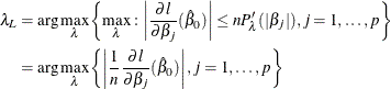
In the GCV approach, the generalized cross validation criteria (GCV) is computed for each value of ![]() on a predetermined grid
on a predetermined grid ![]() ; the value of
; the value of ![]() that achieves the minimum of the GCV is the optimal tuning parameter. The maximum value
that achieves the minimum of the GCV is the optimal tuning parameter. The maximum value ![]() can be determined by lemma 1 in Park and Hastie (2007) as follows. Suppose
can be determined by lemma 1 in Park and Hastie (2007) as follows. Suppose ![]() is free of penalty in the objective function. Let
is free of penalty in the objective function. Let ![]() be the MLE of
be the MLE of ![]() by forcing the rest of the parameters to be zero. Then the maximum value of
by forcing the rest of the parameters to be zero. Then the maximum value of ![]() is
is
You can compute the GCV by using the LASSO framework. In the last step of Newton-Raphson approximation, you have
The solution ![]() satisfies
satisfies
where
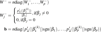
Note that the intercept term has no penalty on its absolute value, and therefore the ![]() term that corresponds to the intercept is 0. More generally, you can make any parameter (such as the
term that corresponds to the intercept is 0. More generally, you can make any parameter (such as the ![]() in the negative binomial model) in the likelihood function free of penalty, and you treat them the same as the intercept.
in the negative binomial model) in the likelihood function free of penalty, and you treat them the same as the intercept.
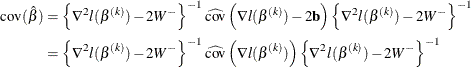
The effective number of parameters is
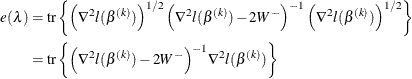
and the generalized cross validation error is
![\begin{align*} e_1 (\lambda ) & = \sum _{j=0}^ p \mathbf{1}_{[\beta _ j \ne 0]}\\ \text {GCV}_1(\lambda )& = \frac{l(\hat{\beta })}{n[1-e_1(\lambda )/n]^2} \end{align*}](images/etsug_countreg0247.png)