The X11 Procedure

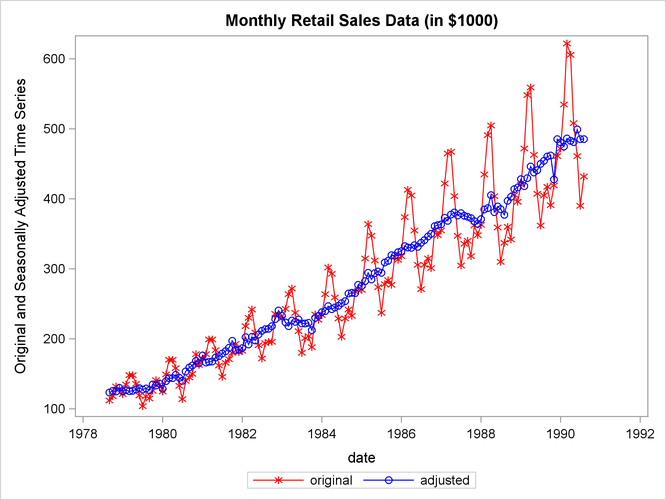
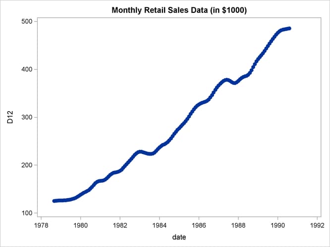
This example computes and plots the final estimates of the individual components for a monthly series. In the first plot (Output 37.1.1), an overlaid plot of the original and seasonally adjusted data is produced. The trend in the data is more evident in the seasonally adjusted data than in the original data. This trend is even more clear in Output 37.1.3, the plot of Table D12, the trend cycle. Note that both the seasonal factors and the irregular factors vary around 100, while the trend cycle and the seasonally adjusted data are in the scale of the original data.

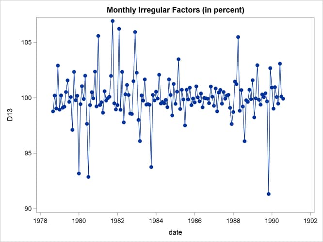
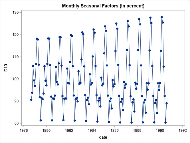
From Output 37.1.2 the seasonal component appears to be slowly increasing, while no apparent pattern exists for the irregular series in Output 37.1.4.

data sales;
   input sales @@;
   date = intnx( 'month', '01sep1978'd, _n_-1 );
   format date monyy7.;
datalines;
112 118 132 129 121 135 148 148 136 119 104 118

   ... more lines ...   

proc x11 data=sales noprint;
   monthly date=date;
   var sales;
   tables b1 d11;
   output out=out b1=series d10=d10 d11=d11
                  d12=d12 d13=d13;
run;

title 'Monthly Retail Sales Data (in $1000)'; 
proc sgplot data=out;
   series x=date y=series / markers
                            markerattrs=(color=red symbol='asterisk')
                            lineattrs=(color=red)
                            legendlabel="original" ;
   series x=date y=d11    / markers
                            markerattrs=(color=blue symbol='circle')
                            lineattrs=(color=blue)
                            legendlabel="adjusted" ;
   yaxis label='Original and Seasonally Adjusted Time Series';
run;

title 'Monthly Seasonal Factors (in percent)'; 
proc sgplot data=out;
   series x=date y=d10 / markers markerattrs=(symbol=CircleFilled) ;
run;

title 'Monthly Retail Sales Data (in $1000)'; 
proc sgplot data=out;
   series x=date y=d12 / markers markerattrs=(symbol=CircleFilled) ;
run;

title 'Monthly Irregular Factors (in percent)'; 
proc sgplot data=out;
   series x=date y=d13 / markers markerattrs=(symbol=CircleFilled) ;
run;