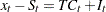
The EXPAND Procedure

Moving Time Window Operators

Some operators compute statistics for a set of values within a moving time window; these are called moving time window operators. There are centered and backward versions of these operators.

The centered moving time window operators are CMOVAVE, CMOVCSS, CMOVGMEAN, CMOVMAX, CMOVMED, CMOVMIN, CMOVPROD, CMOVRANGE, CMOVRANK, CMOVSTD, CMOVSUM, CMOVTVALUE, CMOVUSS, and CMOVVAR. These operators compute statistics of the values for observations

The backward moving time window operators are MOVAVE, MOVCSS, MOVGMEAN, MOVMAX, MOVMED, MOVMIN, MOVPROD, MOVRANGE, MOVRANK, MOVSTD, MOVSUM, MOVTVALUE, MOVUSS, and MOVVAR. These operators compute statistics of the values .

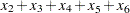
All the moving time window operators accept an argument specifying the number of periods to include in the time window. For example, the following statement computes a five-period backward moving average of X.

   convert x=y / transformout=( movave 5 );

In this example, the resulting transformation is

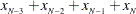
The following statement computes a five-period centered moving average of X.

   convert x=y / transformout=( cmovave 5 );

In this example, the resulting transformation is

If the window with a centered moving time window operator is not an odd number, one more lead value than lag value is included in the time window. For example, the result of the CMOVAVE 4 operator is

You can compute a forward moving time window operation by combining a backward moving time window operator with the REVERSE operator. For example, the following statement computes a five-period forward moving average of X.

   convert x=y / transformout=( reverse movave 5 reverse );

In this example, the resulting transformation is

Some of the moving time window operators enable you to specify a list of weight values to compute weighted statistics. These are CMOVAVE, CMOVCSS, CMOVGMEAN, CMOVPROD, CMOVSTD, CMOVTVALUE, CMOVUSS, CMOVVAR, MOVAVE, MOVCSS, MOVGMEAN, MOVPROD, MOVSTD, MOVTVALUE, MOVUSS, and MOVVAR.

To specify a weighted moving time window operator, enter the weight values in parentheses after the operator name. The window width is equal to the number of weights that you specify; do not specify .

For example, the following statement computes a weighted five-period centered moving average of X.

   convert x=y / transformout=( cmovave( .1 .2 .4 .2 .1 ) );

In this example, the resulting transformation is

The weight values must be greater than zero. If the weights do not sum to 1, the weights specified are divided by their sum to produce the weights used to compute the statistic.

A complete time window is not available at the beginning of the series. For the centered operators a complete window is also not available at the end of the series. The computation of the moving time window operators is adjusted for these boundary conditions as follows.

For backward moving window operators, the width of the time window is shortened at the beginning of the series. For example, the results of the MOVSUM 3 operator are

For centered moving window operators, the width of the time window is shortened at the beginning and the end of the series due to unavailable observations. For example, the results of the CMOVSUM 5 operator are

For weighted moving time window operators, the weights for the unavailable or unused observations are ignored and the remaining weights renormalized to sum to 1.

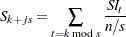
Cumulative Statistics Operators

Some operators compute cumulative statistics for a set of current and previous values of the series. The cumulative statistics operators are CUAVE, CUCSS, CUMAX, CUMED, CUMIN, CURANGE, CUSTD, CUSUM, CUUSS, and CUVAR.

By default, the cumulative statistics operators compute the statistics from all previous values of the series, so that is based on the set of values . For example, the following statement computes as the cumulative sum of nonmissing values for .

   convert x=y / transformout=( cusum );

You can specify a lag increment argument for the cumulative statistics operators. In this case, the statistic is computed from the current and every previous value. When is specified these operators compute statistics of the values for .

For example, the following statement computes as the cumulative sum of nonmissing values for odd when is odd and for even when is even.

   convert x=y / transformout=( cusum 2 );

The results of this example are

Missing Values

You can truncate the length of the result series by using the TRIM, TRIMLEFT, and TRIMRIGHT operators to set values to missing at the beginning or end of the series.

You can use these functions to trim the results of moving time window operators so that the result series contains only values computed from a full width time window. For example, the following statements compute a centered five-period moving average of X, and they set to missing values at the ends of the series that are averages of fewer than five values.

   convert x=y / transformout=( cmovave 5 trim 2 );

Normally, the moving time window and cumulative statistics operators ignore missing values and compute their results for the nonmissing values. When preceded by the NOMISS operator, these functions produce a missing result if any value within the time window is missing.

The NOMISS operator does not perform any calculations, but serves to modify the operation of the moving time window operator that follows it. The NOMISS operator has no effect unless it is followed by a moving time window operator.

For example, the following statement computes a five-period moving average of the variable X but produces a missing value when any of the five values are missing.

   convert x=y / transformout=( nomiss movave 5 );

The following statement computes the cumulative sum of the variable X but produces a missing value for all periods after the first missing X value.

   convert x=y / transformout=( nomiss cusum );

Similar to the NOMISS operator, the MISSONLY operator does not perform any calculations (unless followed by the MEAN option), but it serves to modify the operation of the moving time window operator that follows it. When preceded by the MISSONLY operator, these moving time window operators replace any missing values with the moving statistic and leave nonmissing values unchanged.

For example, the following statement replaces any missing values of the variable X with an exponentially weighted moving average of the past values of X and leaves nonmissing values unchanged. The missing values are interpolated using the specified exponentially weighted moving average. (This is also called simple exponential smoothing.)

   convert x=y / transformout=( missonly ewma 0.3 );

The following statement replaces any missing values of the variable X with the overall mean of X.

   convert x=y / transformout=( missonly mean );

You can use the SETMISS operator to replace missing values with a specified number. For example, the following statement replaces any missing values of the variable X with the number 8.77.

   convert x=y / transformout=( setmiss 8.77 );

Classical Decomposition Operators

If is a seasonal time series with observations per season, classical decomposition methods "break down" the time series into four components: trend, cycle, seasonal, and irregular components. The trend and cycle components are often combined to form the trend-cycle component. There are two basic forms of classical decomposition: multiplicative and additive, which are show below.

where

is the trend-cycle component

is the seasonal component or seasonal factors that are periodic with period and with mean one (multiplicative) or zero (additive)

is the irregular or random component that is assumed to have mean one (multiplicative) or zero (additive)

For multiplicative decomposition, all of the values should be positive.

The CD_TC operator computes the trend-cycle component for both the multiplicative and additive models. When is odd, this operator computes an -period centered moving average as follows:

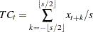For example, in the case where s=5, the CD_TC s operator

   convert x=tc / transformout=( cd_tc 5 );

is equivalent to the following CMOVAVE operator:

   convert x=tc / transformout=( cmovave 5 trim 2 );

When is even, the CD_TC s operator computes the average of two adjacent -period centered moving averages as follows:

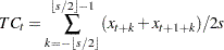For example, in the case where s=12, the CD_TC s operator

   convert x=tc / transformout=( cd_tc 12 );

is equivalent to the following CMOVAVE operator:

   convert x=tc / transformout=(cmovave 12 movave 2 trim 6);

The CD_S and CDA_S operators compute the seasonal components for the multiplicative and additive models, respectively. First, the trend-cycle component is computed as shown previously. Second, the seasonal-irregular component is computed by for the multiplicative model and by for the additive model. The seasonal component is obtained by averaging the seasonal-irregular component for each season.

where and . The seasonal components are normalized to sum to one (multiplicative) or zero (additive).

The CD_I and CDA_I operators compute the irregular component for the multiplicative and additive models respectively. First, the seasonal component is computed as shown previously. Next, the irregular component is determined from the seasonal-irregular and seasonal components as appropriate.

The CD_SA and CDA_SA operators compute the seasonally adjusted time series for the multiplicative and additive models, respectively. After decomposition, the original time series can be seasonally adjusted as appropriate.

The following statements compute all the multiplicative classical decomposition components for the variable X for =12.

   convert x=tc / transformout=( cd_tc 12 );
   convert x=s  / transformout=( cd_s  12 );
   convert x=i  / transformout=( cd_i  12 );
   convert x=sa / transformout=( cd_sa 12 );

The following statements compute all the additive classical decomposition components for the variable X for =4.

   convert x=tc / transformout=( cd_tc  4 );
   convert x=s  / transformout=( cda_s  4 );
   convert x=i  / transformout=( cda_i  4 );
   convert x=sa / transformout=( cda_sa 4 );

The X12 and X11 procedures provides other methods for seasonal decomposition. See Chapter 37, The X12 Procedure, and Chapter 36, The X11 Procedure.

Fractional Operators

For fractional operators, the parameter, d, represents the order of fractional differencing. Fractional summation is the inverse operation of fractional differencing.

   convert x=y / transformout=(fdif 0.25);

   convert z=w / transformout=(fsum 0.25);

Moving Rank Operators

For the rank operators, the ranks are computed based on the current value with respect to the cumulative, centered, or moving window values. If the current value is missing, the transformed current value is set to missing. If the NOMISS option was previously specified and if any missing values are present in the moving window, the transformed current value is set to missing. Otherwise, redundant values from the moving window are removed and the rank of the current value is computed among the unique values of the moving window.

   convert price=history / transformout=( curank );

   convert price=lastweek / transformout=( movrank 5 );

   convert price=twoweek / transformout=( movrank 10 );

Moving Product and Geometric Mean Operators

For the product and geometric mean operators, the current transformed value is computed based on the (weighted) product of the cumulative, centered, or moving window values. If missing values are present in the moving window and the NOMISS operator is previously specified, the current transformed value is set to missing. Otherwise, the current transformed value is set to the product of the nonmissing values within the moving window. If a geometric mean operator is specified for a window of size , the root of the product is taken. In cases where weights are specified explicitly, both the product and geometric mean operators normalize these exponents so that they sum to one.

   convert rates=history / transformout=( + 1 cuprod - 1);

   convert rates=lastqtr / transformout=( + 1 movprod 3 - 1);

   convert rates=lastqtr / transformout=( + 1 movprod (1 1 1) - 1);

Sequence Operators

For the sequence operators, the sequence values are used to compute the transformed values from the original values in a sequential fashion. You can add to or subtract from the original series or you can multiply or divide by the sequence values. The first sequence value is applied to the first observation of the series, the second sequence value is applied to the second observation of the series, and so on until the end of the sequence is reached. At this point, the first sequence value is applied to the next observation of the series and the second sequence value on the next observation and so on.

Let be the sequence values and let , , be the original time series. The transformed series, , is computed as follows:

where .

   convert seasadj=seasonal /
           transformout=(seqmult (0.9 1.2 0.8 1.1));

   convert seasadj=seasonal /
           transformout=(seqadd (4.4 -1.1 -2.1 -1.2));

Set Operators

For the set operators, the first parameter, , represents the value to be replaced and the second parameter, , represents the replacement value. The replacement can be localized to the beginning, middle, or end of the series.

   convert sales=demand / transformout=(setleft (0 .));

   convert sales=demand / transformout=(setright (0 .));

Scale Operator

For the scale operator, the first parameter, , represents the value associated with the minimum value () and the second parameter, , represents the value associated with the maximum value () of the original series (). The scale operator recales the original data to be between the parameters and as follows:

   convert x=w / transformout=(scale 0 1);
   convert y=z / transformout=(scale 0 1);

Adjust Operator

For the moving summation and product window operators, the window widths at the beginning and end of the series are smaller than those in the middle of the series. Likewise, if there are embedded missing values, the window width is smaller than specified. When preceded by the ADJUST operator, the moving summation (MOVSUM CMOVSUM) and moving product operators (MOVPROD CMOVPROD) are adjusted by the window width.

For example, suppose the variable has 10 values and the moving summation operator of width 3 is applied to to create the variable with window width adjustment and the variable without adjustment.

   convert x=y / transformout=(adjust movsum 3);
   convert x=z / transformout=(movsum 3);

The above transformations result in the following relationship between and : , , for because the first two window widths are smaller than 3.

For example, suppose the variable has 10 values and the moving multiplicative operator of width 3 is applied to to create the variable with window width adjustment and the variable without adjustment.

   convert x=y / transformout=(adjust movprod 3);
   convert x=z / transformout=(movprod 3);

The above transformation result in the following: , , for because the first two window widths are smaller than 3.

Moving T-Value Operators

The moving t-value operators (CUTVALUE, MOVTVALUE, CMOVTVALUE) compute the t-value of the cumulative series or moving window. They can be viewed as combinations of the moving average (CUAVE, MOVAVE, CMOVAVE) and the moving standard deviation (CUSTD, MOVSTD, CMOVSTD), respectively.

Percent Operators

The percentage operators compute the percent summation and the percent difference of the current value and the . The percent summation operator (PCTSUM) computes 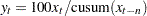. If any of the values of the preceding equation are missing or the cumulative summation is zero, the result is set to missing. The percent difference operator (PCTDIF) computes . If any of the values of the preceding equation are missing or the lag value is zero, the result is set to missing.

For example, suppose variable contains the series. The percent summation of lag 4 is applied to to create the variable . The percent difference of lag 4 is applied to to create the variable .

   convert x=y / transformout=(pctsum 4);
   convert x=z / transformout=(pctdif 4);

Ratio Operators

The ratio operator computes the ratio of the current value and the value. The ratio operator (RATIO) computes . If any of the values of the preceding equation are missing or the lag value is zero, the result is set to missing.

For example, suppose variable contains the series. The ratio of the current value and the lag 4 value of assigned to the variable . The percent ratio of the current value and lag 4 value of is assigned to the variable .

   convert x=y / transformout=(ratio 4);
   convert x=z / transformout=(ratio 4 * 100);