The ARIMA Procedure

Statistical procedures use ODS Graphics to create graphs as part of their output. ODS Graphics is described in detail in Chapter 21, Statistical Graphics Using ODS (SAS/STAT User's Guide).

Before you create graphs, ODS Graphics must be enabled (for example, with the ODS GRAPHICS ON statement). For more information about enabling and disabling ODS Graphics, see the section "Enabling and Disabling ODS Graphics" in that chapter.

The overall appearance of graphs is controlled by ODS styles. Styles and other aspects of using ODS Graphics are discussed in the section "A Primer on ODS Statistical Graphics" in that chapter.

This section provides information about the graphics produced by the ARIMA procedure. (See Chapter 21, Statistical Graphics Using ODS (SAS/STAT User's Guide), for more information about ODS statistical graphics.) The main types of plots available are as follows:

• plots useful in the trend and correlation analysis of the dependent and input series

• plots useful for the residual analysis of an estimated model

• forecast plots

You can obtain most plots relevant to the specified model by default. For finer control of the graphics, you can use the PLOTS= option in the PROC ARIMA statement. The following example is a simple illustration of how to use the PLOTS= option.

Airline Series: Illustration of ODS Graphics

The series in this example, the monthly airline passenger series, is also discussed later, in Example 7.2.

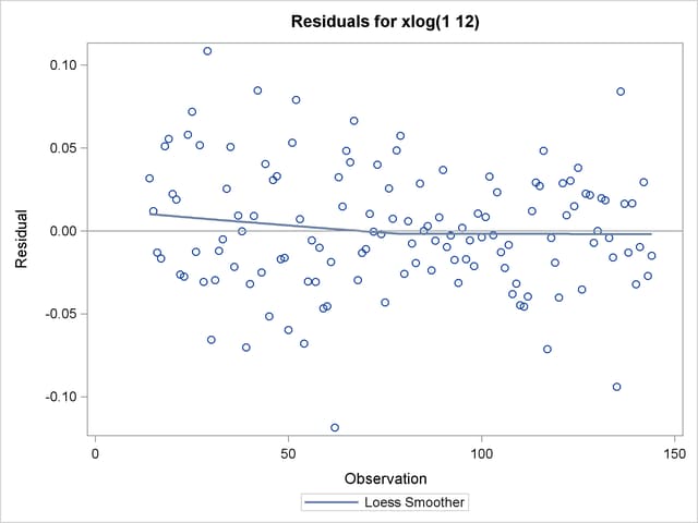
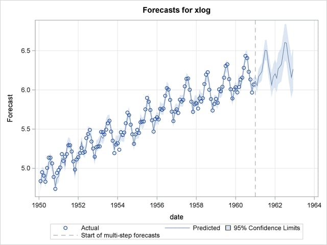
The following statements specify an ARIMA(0,1,1)(0,1,1) model without a mean term to the logarithms of the airline passengers series, xlog. Notice the use of the global plot option ONLY in the PLOTS= option of the PROC ARIMA statement. It suppresses the production of default graphics and produces only the plots specified by the subsequent RESIDUAL and FORECAST plot options. The RESIDUAL(SMOOTH) plot specification produces a time series plot of residuals that has an overlaid loess fit; see Figure 7.21. The FORECAST(FORECAST) option produces a plot that shows the one-step-ahead forecasts, as well as the multistep-ahead forecasts; see Figure 7.22.

proc arima data=seriesg 
   plots(only)=(residual(smooth) forecast(forecasts));
   identify var=xlog(1,12);
   estimate q=(1)(12) noint method=ml;
   forecast id=date interval=month;
run;

Figure 7.21 Residual Plot of the Airline Model

Figure 7.22 Forecast Plot of the Airline Model