| The MODEL Procedure |
| Heteroscedasticity |
One of the key assumptions of regression is that the variance of the errors is constant across observations. If the errors have constant variance, the errors are called homoscedastic. Typically, residuals are plotted to assess this assumption. Standard estimation methods are inefficient when the errors are heteroscedastic or have nonconstant variance.
Heteroscedasticity Tests
The MODEL procedure provides two tests for heteroscedasticity of the errors: White’s test and the modified Breusch-Pagan test.
Both White’s test and the Breusch-Pagan are based on the residuals of the fitted model. For systems of equations, these tests are computed separately for the residuals of each equation.
The residuals of an estimation are used to investigate the heteroscedasticity of the true disturbances.
The WHITE option tests the null hypothesis
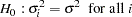 |
White’s test is general because it makes no assumptions about the form of the heteroscedasticity (White 1980). Because of its generality, White’s test might identify specification errors other than heteroscedasticity (Thursby 1982). Thus, White’s test might be significant when the errors are homoscedastic but the model is misspecified in other ways.
White’s test is equivalent to obtaining the error sum of squares for the regression of squared residuals on a constant and all the unique variables in  , where the matrix J is composed of the partial derivatives of the equation residual with respect to the estimated parameters. White’s test statistic
  is computed as follows:
 |
where  is the correlation coefficient obtained from the above regression. The statistic is asymptotically distributed as chi-squared with P–1 degrees of freedom, where P is the number of regressors in the regression, including the constant and n is the total number of observations. In the example given below, the regressors are constant, income, income*income, income*income*income, and income*income*income*income. income*income occurs twice and one is dropped. Hence, P=5 with degrees of freedom, P–1=4.
Note that White’s test in the MODEL procedure is different than White’s test in the REG procedure requested by the SPEC option. The SPEC option produces the test from Theorem 2 on page 823 of White (1980). The WHITE option, on the other hand, produces the statistic discussed in Greene (1993).
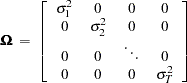
The null hypothesis for the modified Breusch-Pagan test is homosedasticity. The alternate hypothesis is that the error variance varies with a set of regressors, which are listed in the BREUSCH= option.
Define the matrix  to be composed of the values of the variables listed in the BREUSCH= option, such that
  is the value of the jth variable in the BREUSCH= option for the ith observation. The null hypothesis of the Breusch-Pagan test is
 |
where  is the error variance for the ith observation and
  and
and  are regression coefficients.
The test statistic for the Breusch-Pagan test is
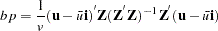 |
where 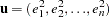 ,
,  is a
is a  vector of ones, and
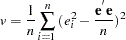 |
This is a modified version of the Breusch-Pagan test, which is less sensitive to the assumption of normality than the original test (Greene 1993, p. 395).
The statements in the following example produce the output in Figure 18.39:
   proc model data=schools;
      parms const inc inc2;

      exp = const + inc * income + inc2 * income * income;
      incsq = income * income;

      fit exp / white breusch=(1 income incsq);
   run;
| Heteroscedasticity Test | |||||
|---|---|---|---|---|---|
| Equation | Test | Statistic | DF | Pr > ChiSq | Variables |
| exp | White's Test | 21.16 | 4 | 0.0003 | Cross of all vars |
| Breusch-Pagan | 15.83 | 2 | 0.0004 | 1, income, incsq | |
Correcting for Heteroscedasticity
There are two methods for improving the efficiency of the parameter estimation in the presence of heteroscedastic errors. If the error variance relationships are known, weighted regression can be used or an error model can be estimated. For details about error model estimation, see the section Error Covariance Structure Specification. If the error variance relationship is unknown, GMM estimation can be used.
Weighted Regression
The WEIGHT statement can be used to correct for the heteroscedasticity. Consider the following model, which has a heteroscedastic error term:
 |
The data for this model is generated with the following SAS statements.
   data test;
      do t=1 to 25;
         y = 250 * (exp( -0.2 * t ) - exp( -0.8 * t )) +
             sqrt( 9 / t ) * rannor(1);
         output;
      end;
   run;
If this model is estimated with OLS, as shown in the following statements, the estimates shown in Figure 18.40 are obtained for the parameters.
   proc model data=test;
      parms b1 0.1 b2 0.9;
      y = 250 * ( exp( -b1 * t ) - exp( -b2 * t ) );
      fit y;
   run;
| Nonlinear OLS Parameter Estimates | ||||
|---|---|---|---|---|
| Parameter | Estimate | Approx Std Err | t Value | Approx Pr > |t| |
| b1 | 0.200977 | 0.00101 | 198.60 | <.0001 |
| b2 | 0.826236 | 0.00853 | 96.82 | <.0001 |
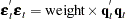
If both sides of the model equation are multiplied by  , the model has a homoscedastic error term. This multiplication or weighting is done through the WEIGHT statement. The WEIGHT statement variable operates on the squared residuals as
 |
so that the WEIGHT statement variable represents the square of the model multiplier. The following PROC MODEL statements corrects the heteroscedasticity with a WEIGHT statement:
   proc model data=test;
      parms b1 0.1 b2 0.9;
      y = 250 * ( exp( -b1 * t ) - exp( -b2 * t ) );
      fit y;
      weight t;
   run;
Note that the WEIGHT statement follows the FIT statement. The weighted estimates are shown in Figure 18.41.
The weighted OLS estimates are identical to the output produced by the following PROC MODEL example:
   proc model data=test;
      parms b1 0.1 b2 0.9;
      y = 250 * ( exp( -b1 * t ) - exp( -b2 * t ) );
     _weight_ = t;
      fit y;
   run;
If the WEIGHT statement is used in conjunction with the _WEIGHT_ variable, the two values are multiplied together to obtain the weight used.
The WEIGHT statement and the _WEIGHT_ variable operate on all the residuals in a system of equations. If a subset of the equations needs to be weighted, the residuals for each equation can be modified through the RESID. variable for each equation. The following example demonstrates the use of the RESID. variable to make a homoscedastic error term:
   proc model data=test;
      parms b1 0.1 b2 0.9;
      y = 250 * ( exp( -b1 * t ) - exp( -b2 * t ) );
      resid.y = resid.y * sqrt(t);
      fit y;
   run;
These statements produce estimates of the parameters and standard errors that are identical to the weighted OLS estimates. The reassignment of the RESID.Y variable must be done after Y is assigned; otherwise it would have no effect. Also, note that the residual (RESID.Y) is multiplied by . Here the multiplier is acting on the residual before it is squared.
GMM Estimation
If the form of the heteroscedasticity is unknown, generalized method of moments estimation (GMM) can be used. The following PROC MODEL statements use GMM to estimate the example model used in the preceding section:
   proc model data=test;
      parms b1 0.1 b2 0.9;
      y = 250 * ( exp( -b1 * t ) - exp( -b2 * t ) );
      fit y / gmm;
      instruments b1 b2;
   run;
GMM is an instrumental method, so instrument variables must be provided.
GMM estimation generates estimates for the parameters shown in Figure 18.42.
| Nonlinear GMM Parameter Estimates | ||||
|---|---|---|---|---|
| Parameter | Estimate | Approx Std Err | t Value | Approx Pr > |t| |
| b1 | 0.200487 | 0.000800 | 250.69 | <.0001 |
| b2 | 0.822148 | 0.0148 | 55.39 | <.0001 |
Heteroscedasticity-Consistent Covariance Matrix Estimation
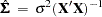
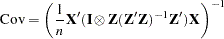
Homoscedasticity is required for ordinary least squares regression estimates to be efficient. A nonconstant error variance, heteroscedasticity, causes the OLS estimates to be inefficient, and the usual OLS covariance matrix,  , is generally invalid:
 |
When the variance of the errors of a classical linear model
 |
is not constant across observations (heteroscedastic), so that  for some
  , the OLS estimator
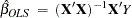 |
is unbiased but it is inefficient. Models that take into account the changing variance can make more efficient use of the data. When the variances,  , are known, generalized least squares (GLS) can be used and the estimator
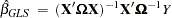 |
where
 |
is unbiased and efficient. However, GLS is unavailable when the variances,  , are unknown.
To solve this problem White (1980) proposed a heteroscedastic consistent-covariance matrix estimator (HCCME)
 |
that is consistent as well as unbiased, where
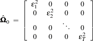 |
and 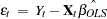 .
.
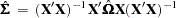
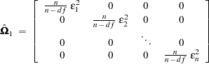
This estimator is considered somewhat unreliable in finite samples. Therefore, Davidson and MacKinnon (1993) propose three different modifications to estimating  . The first solution is to simply multiply
  by
by  , where n is the number of observations and df is the number of explanatory variables, so that
 |
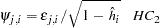
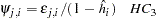
The second solution is to define
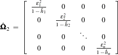 |
where 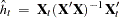 .
.
The third solution, called the "jackknife," is to define
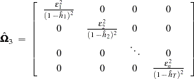 |
MacKinnon and White (1985) investigated these three modified HCCMEs, including the original HCCME, based on finite-sample performance of pseudo- statistics. The original HCCME performed the worst. The first modification performed better. The second modification performed even better than the first, and the third modification performed the best. They concluded that the original HCCME should never be used in finite sample estimation, and that the second and third modifications should be used over the first modification if the diagonals of are available.
Seemingly Unrelated Regression HCCME
Extending the discussion to systems of  equations, the HCCME for SUR estimation is
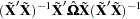 |
where  is a
is a  matrix with the first rows representing the first observation, the next rows representing the second observation, and so on.
  is now a
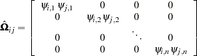
  block diagonal matrix with typical block
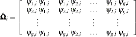 |
where
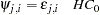 |
or
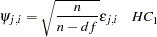 |
or
 |
or
 |
Two- and Three-Stage Least Squares HCCME
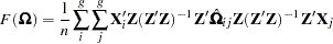
For two- and three-stage least squares, the HCCME for a equation system is
 |
where
 |
is the normal covariance matrix without the  matrix and
 |
where  is a
is a  matrix with the
  th equations regressors in the appropriate columns and zeros everywhere else.
 |
For 2SLS  when
when  . The
. The  used in is computed by using the parameter estimates obtained from the instrumental variables estimation.
The leverage value for the  th equation used in the HCCME=2 and HCCME=3 methods is computed as conditional on the first stage as
 |
for 2SLS and
 |
for 3SLS.
Copyright © 2008 by SAS Institute Inc., Cary, NC, USA. All rights reserved.