| The MODEL Procedure |
| Testing for Normality |
The NORMAL option in the FIT statement performs multivariate and univariate tests of normality.
The three multivariate tests provided are Mardia’s skewness test and kurtosis test (Mardia 1970) and the Henze-Zirkler  test (Henze and Zirkler 1990). The two univariate tests provided are the Shapiro-Wilk W test and the Kolmogorov-Smirnov test. (For details on the univariate tests, refer to "Goodness-of-Fit Tests" section in "The UNIVARIATE Procedure" chapter in the Base SAS Procedures Guide.) The null hypothesis for all these tests is that the residuals are normally distributed.
For a random sample  ,
,  , where d is the dimension of
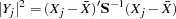
  and n is the number of observations, a measure of multivariate skewness is
 |
where S is the sample covariance matrix of X. For weighted regression, both S and  are computed by using the weights supplied by the WEIGHT statement or the _WEIGHT_ variable.
Mardia showed that under the null hypothesis  is asymptotically distributed as
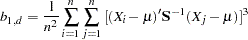
 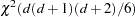 . For small samples, Mardia’s skewness test statistic is calculated with a small sample correction formula, given by
  where the correction factor
  is given by
  . Mardia’s skewness test statistic in PROC MODEL uses this small sample corrected formula.
A measure of multivariate kurtosis is given by
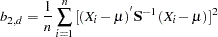 |
Mardia showed that under the null hypothesis,  is asymptotically normally distributed with mean
  and variance
  .
.
The Henze-Zirkler test is based on a nonnegative functional  that measures the distance between two distribution functions and has the property that
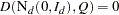 |
if and only if
 |
where  is a d-dimensional normal distribution.
The distance measure can be written as
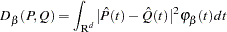 |
where  and
and  are the Fourier transforms of P and Q, and
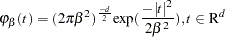
  is a weight or a kernel function. The density of the normal distribution
  is used as
 |
where  .
.
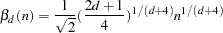
The parameter  depends on
  as
as
 |
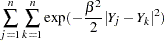
The test statistic computed is called  and is approximately distributed as a lognormal. The lognormal distribution is used to compute the null hypothesis probability.
 |
 |
 |
|||
 |
 |
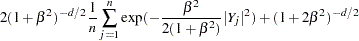 |
where
 |
 |
Monte Carlo simulations suggest that has good power against distributions with heavy tails.
The Shapiro-Wilk W test is computed only when the number of observations (n ) is less than  while computation of the Kolmogorov-Smirnov test statistic requires at least observations.
The following is an example of the output produced by the NORMAL option.
   proc model data=test2;
      y1 = a1 * x2 * x2 - exp( d1*x1);
      y2 = a2 * x1 * x1 + b2 * exp( d2*x2);
      fit y1 y2 / normal ;
   run;
| Normality Test | |||
|---|---|---|---|
| Equation | Test Statistic | Value | Prob |
| y1 | Shapiro-Wilk W | 0.37 | <.0001 |
| y2 | Shapiro-Wilk W | 0.84 | <.0001 |
| System | Mardia Skewness | 286.4 | <.0001 |
| Mardia Kurtosis | 31.28 | <.0001 | |
| Henze-Zirkler T | 7.09 | <.0001 | |
Copyright © 2008 by SAS Institute Inc., Cary, NC, USA. All rights reserved.