| The MDC Procedure |
| Nested Logit Modeling |
A more general model can be specified using the nested logit model.
Consider, for example, the following random utility function:
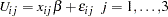 |
Suppose the set of all alternatives indexed by  is partitioned into
  nests,
  . The nested logit model is obtained by assuming that the error term in the utility function has the GEV cumulative distribution function:
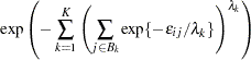 |
where  is a measure of a degree of independence among the alternatives in nest
  . When
  for all , the model reduces to the standard logit model.
Since the public transportation modes, 1 and 2, tend to be correlated, these two choices can be grouped together. The decision tree displayed in Figure 17.8 is constructed.
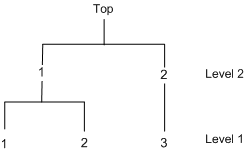
The two-level decision tree is specified in the NEST statement. The NCHOICE= option is not allowed for nested logit estimation. Instead, the CHOICE= option needs to be specified, as in the following statements:
   /*-- nested logit estimation --*/
   proc mdc data=newdata;
      model decision = ttime /
               type=nlogit
               choice=(mode 1 2 3)
               covest=hess;
      id pid;
      utility u(1,) = ttime;
      nest level(1) = (1 2 @ 1, 3 @ 2),
           level(2) = (1 2 @ 1);
   run;
In Figure 17.9, estimates of the inclusive value parameters, INC_L2G1C1 and INC_L2G1C2, are indicative of a nested model structure. See the section Nested Logit and the section Decision Tree and Nested Logit for more details on inclusive values.
| Parameter Estimates | |||||
|---|---|---|---|---|---|
| Parameter | DF | Estimate | Standard Error |
t Value | Approx Pr > |t| |
| ttime_L1 | 1 | -0.4040 | 0.1241 | -3.25 | 0.0011 |
| INC_L2G1C1 | 1 | 0.8016 | 0.4352 | 1.84 | 0.0655 |
| INC_L2G1C2 | 1 | 0.8087 | 0.3591 | 2.25 | 0.0243 |
The nested logit model is estimated with the restriction INC_L2G1C1 =INC_L2G1C2 by specifying the SAMESCALE option, as in the following statements. The estimation result is displayed in Figure 17.10.
   /*-- nlogit with samescale option --*/
   proc mdc data=newdata;
      model decision = ttime /
               type=nlogit
               choice=(mode 1 2 3)
               samescale
               covest=hess;
      id pid;
      utility u(1,) = ttime;
      nest level(1) = (1 2 @ 1, 3 @ 2),
           level(2) = (1 2 @ 1);
   run;
| Parameter Estimates | |||||
|---|---|---|---|---|---|
| Parameter | DF | Estimate | Standard Error |
t Value | Approx Pr > |t| |
| ttime_L1 | 1 | -0.4025 | 0.1217 | -3.31 | 0.0009 |
| INC_L2G1 | 1 | 0.8209 | 0.3019 | 2.72 | 0.0066 |
The nested logit model is equivalent to the conditional logit model if INC_L2G1C1 = INC_L2G1C2 = 1. You can verify this relationship by estimating a constrained nested logit model. (See the section RESTRICT Statement for details on imposing linear restrictions on parameter estimates.) The parameter estimates and the active linear constraints for the following constrained nested logit model are displayed in Figure 17.11.
   /*-- constrained nested logit estimation --*/
   proc mdc data=newdata;
      model decision = ttime /
               type=nlogit
               choice=(mode 1 2 3)
               covest=hess;
      id pid;
      utility u(1,) = ttime;
      nest level(1) = (1 2 @ 1, 3 @ 2),
           level(2) = (1 2 @ 1);
      restrict INC_L2G1C1 = 1, INC_L2G1C2 =1;
   run;
| Parameter Estimates | ||||||
|---|---|---|---|---|---|---|
| Parameter | DF | Estimate | Standard Error |
t Value | Approx Pr > |t| |
Parameter Label |
| ttime_L1 | 1 | -0.3572 | 0.0776 | -4.60 | <.0001 | |
| INC_L2G1C1 | 0 | 1.0000 | 0 | |||
| INC_L2G1C2 | 0 | 1.0000 | 0 | |||
| Restrict1 | 1 | -2.1706 | 8.4098 | -0.26 | 0.7993* | Linear EC [ 1 ] |
| Restrict2 | 1 | 3.6573 | 10.0001 | 0.37 | 0.7186* | Linear EC [ 2 ] |
| Linearly Independent Active Linear Constraints | |||||||
|---|---|---|---|---|---|---|---|
| 1 | 0 | = | -1.0000 | + | 1.0000 | * | INC_L2G1C1 |
| 2 | 0 | = | -1.0000 | + | 1.0000 | * | INC_L2G1C2 |
Copyright © 2008 by SAS Institute Inc., Cary, NC, USA. All rights reserved.