Consider the following linear regression model:

where is an data matrix, is a coefficient vector, and is a disturbance vector. The error term is assumed to be generated by the th-order autoregressive process where , is a sequence of independent normal error terms with mean 0 and variance . Usually, the Durbin-Watson statistic is used to test the null hypothesis against . Vinod (1973) generalized the Durbin-Watson statistic:

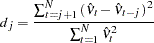where are OLS residuals. Using the matrix notation,

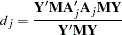where 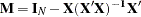and is a matrix:

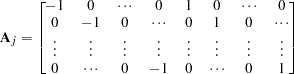and there are zeros between and 1 in each row of matrix .

The QR factorization of the design matrix yields a orthogonal matrix :

where R is an upper triangular matrix. There exists an submatrix of such that and . Consequently, the generalized Durbin-Watson statistic is stated as a ratio of two quadratic forms:

where are upper n eigenvalues of and is a standard normal variate, and . These eigenvalues are obtained by a singular value decomposition of (Golub and Van Loan; 1989; Savin and White; 1978).

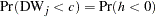
The marginal probability (or p-value) for given is

where

When the null hypothesis holds, the quadratic form has the characteristic function

The distribution function is uniquely determined by this characteristic function:

For example, to test given against , the marginal probability (p-value) can be used:

where

and is the calculated value of the fourth-order Durbin-Watson statistic.

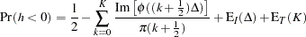
In the Durbin-Watson test, the marginal probability indicates positive autocorrelation () if it is less than the level of significance (), while you can conclude that a negative autocorrelation () exists if the marginal probability based on the computed Durbin-Watson statistic is greater than . Wallis (1972) presented tables for bounds tests of fourth-order autocorrelation, and Vinod (1973) has given tables for a 5% significance level for orders two to four. Using the AUTOREG procedure, you can calculate the exact p-values for the general order of Durbin-Watson test statistics. Tests for the absence of autocorrelation of order p can be performed sequentially; at the th step, test given against . However, the size of the sequential test is not known.

The Durbin-Watson statistic is computed from the OLS residuals, while that of the autoregressive error model uses residuals that are the difference between the predicted values and the actual values. When you use the Durbin-Watson test from the residuals of the autoregressive error model, you must be aware that this test is only an approximation. See Autoregressive Error Model earlier in this chapter. If there are missing values, the Durbin-Watson statistic is computed using all the nonmissing values and ignoring the gaps caused by missing residuals. This does not affect the significance level of the resulting test, although the power of the test against certain alternatives may be adversely affected. Savin and White (1978) have examined the use of the Durbin-Watson statistic with missing values.

Enhanced Durbin-Watson Probability Computation

The Durbin-Watson probability calculations have been enhanced to compute the -value of the generalized Durbin-Watson statistic for large sample sizes. Previously, the Durbin-Watson probabilities were only calculated for small sample sizes.

Consider the following linear regression model:

where is an data matrix, is a coefficient vector, is a disturbance vector, and is a sequence of independent normal error terms with mean 0 and variance .

The generalized Durbin-Watson statistic is written as

where is a vector of OLS residuals and is a matrix. The generalized Durbin-Watson statistic DW can be rewritten as

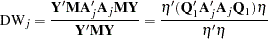where .

The marginal probability for the Durbin-Watson statistic is

where .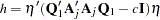

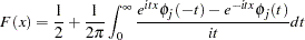
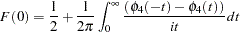
The -value or the marginal probability for the generalized Durbin-Watson statistic is computed by numerical inversion of the characteristic function of the quadratic form . The trapezoidal rule approximation to the marginal probability is

where is the imaginary part of the characteristic function, and are integration and truncation errors, respectively. Refer to Davies (1973) for numerical inversion of the characteristic function.

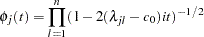
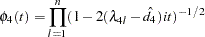
Ansley, Kohn, and Shively (1992) proposed a numerically efficient algorithm that requires O() operations for evaluation of the characteristic function . The characteristic function is denoted as

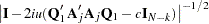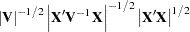where 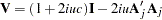and . By applying the Cholesky decomposition to the complex matrix , you can obtain the lower triangular matrix that satisfies . Therefore, the characteristic function can be evaluated in O() operations by using the following formula:

where . Refer to Ansley, Kohn, and Shively (1992) for more information on evaluation of the characteristic function.

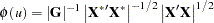
Tests for Serial Correlation with Lagged Dependent Variables

When regressors contain lagged dependent variables, the Durbin-Watson statistic () for the first-order autocorrelation is biased toward 2 and has reduced power. Wallis (1972) shows that the bias in the Durbin-Watson statistic () for the fourth-order autocorrelation is smaller than the bias in in the presence of a first-order lagged dependent variable. Durbin (1970) proposes two alternative statistics (Durbin h and t ) that are asymptotically equivalent. The h statistic is written as

where and is the least squares variance estimate for the coefficient of the lagged dependent variable. Durbin’s t test consists of regressing the OLS residuals on explanatory variables and and testing the significance of the estimate for coefficient of .

Inder (1984) shows that the Durbin-Watson test for the absence of first-order autocorrelation is generally more powerful than the h test in finite samples. Refer to Inder (1986) and King and Wu (1991) for the Durbin-Watson test in the presence of lagged dependent variables.