Heteroscedasticity and Normality Tests

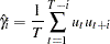
Portmanteau Q Test

For nonlinear time series models, the portmanteau test statistic based on squared residuals is used to test for independence of the series (McLeod and Li; 1983):

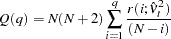where

This Q statistic is used to test the nonlinear effects (for example, GARCH effects) present in the residuals. The GARCH process can be considered as an ARMA process. See the section Predicting the Conditional Variance later in this chapter. Therefore, the Q statistic calculated from the squared residuals can be used to identify the order of the GARCH process.

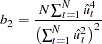
Lagrange Multiplier Test for ARCH Disturbances

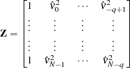
Engle (1982) proposed a Lagrange multiplier test for ARCH disturbances. The test statistic is asymptotically equivalent to the test used by Breusch and Pagan (1979). Engle’s Lagrange multiplier test for the qth order ARCH process is written

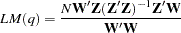where

and

The presample values ( ,, ) have been set to 0. Note that the LM tests may have different finite-sample properties depending on the presample values, though they are asymptotically equivalent regardless of the presample values. The LM and Q statistics are computed from the OLS residuals assuming that disturbances are white noise. The Q and LM statistics have an approximate distribution under the white-noise null hypothesis.

Normality Test

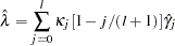
Based on skewness and kurtosis, Jarque and Bera (1980) calculated the test statistic

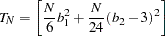where

The (2) distribution gives an approximation to the normality test .

When the GARCH model is estimated, the normality test is obtained using the standardized residuals . The normality test can be used to detect misspecification of the family of ARCH models.

Computation of the Chow Test

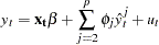
Consider the linear regression model

where the parameter vector contains elements.

Split the observations for this model into two subsets at the break point specified by the CHOW= option, so that

Now consider the two linear regressions for the two subsets of the data modeled separately,

where the number of observations from the first set is and the number of observations from the second set is .

The Chow test statistic is used to test the null hypothesis conditional on the same error variance . The Chow test is computed using three sums of square errors:

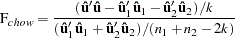where is the regression residual vector from the full set model, is the regression residual vector from the first set model, and is the regression residual vector from the second set model. Under the null hypothesis, the Chow test statistic has an F distribution with and degrees of freedom, where is the number of elements in .

Chow (1960) suggested another test statistic that tests the hypothesis that the mean of prediction errors is 0. The predictive Chow test can also be used when .

The PCHOW= option computes the predictive Chow test statistic

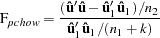The predictive Chow test has an F distribution with and degrees of freedom.

Phillips-Perron Unit Root and Cointegration Testing

Consider the random walk process

where the disturbances might be serially correlated with possible heteroscedasticity. Phillips and Perron (1988) proposed the unit root test of the OLS regression model,

Let 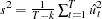and let be the variance estimate of the OLS estimator , where is the OLS residual. You can estimate the asymptotic variance of by using the truncation lag l.

where , for , and .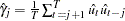

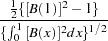
Then the Phillips-Perron (defined here as ) test (zero mean case) is written

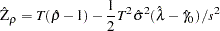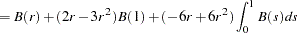
and has the following limiting distribution:

where B() is a standard Brownian motion. Note that the realization from the stochastic process is distributed as and thus .

Note that as , which shows that the limiting distribution is skewed to the left.

Let be the statistic for . The Phillips-Perron (defined here as ) test is written

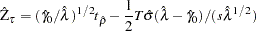and its limiting distribution is derived as

When you test the regression model 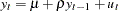for the true random walk process (single mean case), the limiting distribution of the statistic is written

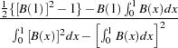while the limiting distribution of the statistic is given by

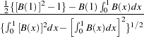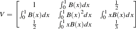
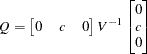
Finally, the limiting distribution of the Phillips-Perron test for the random walk with drift process 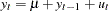(trend case) can be derived as

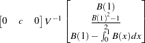where for and for ,

When several variables are cointegrated, there exists a cointegrating vector such that is stationary and is a nonzero vector. The residual based cointegration test assumes the following regression model:

where , , and = (,,. You can estimate the consistent cointegrating vector by using OLS if all variables are difference stationary — that is, I(1). The Phillips-Ouliaris test is computed using the OLS residuals from the preceding regression model, and it performs the test for the null hypothesis of no cointegration. The estimated cointegrating vector is .

You need to refer to the tables by Phillips and Ouliaris (1990) to obtain the -value of the cointegration test. Before you apply the cointegration test, you may want to perform the unit root test for each variable (see the option STATIONARITY= ( PHILLIPS )).

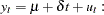
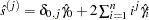
Kwiatkowski, Phillips, Schmidt, and Shin (KPSS) Unit Root Test

The KPSS test was introduced in Kwiatkowski et al. (1992) to test the null hypothesis that an observable series is stationary around a deterministic trend. Please note, that for consistency reasons, the notation used here is different from the notation used in the original paper. The setup of the problem is as follows: it is assumed that the series is expressed as the sum of the deterministic trend, random walk , and stationary error ; that is,

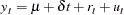with , iid , and an intercept (in the original paper, the authors use instead of .) Under stronger assumptions of normality and iid of and , a one-sided LM test of the null that there is no random walk () can be constructed as follows:

Following the original work of Kwiatkowski, Phillips, Schmidt, and Shin, under the null (), statistic converges asymptotically to three different distributions depending on whether the model is trend-stationary, level-stationary (), or zero-mean stationary (, ). The trend-stationary model is denoted by subscript and the level-stationary model is denoted by subscript . The case when there is no trend and zero intercept denoted as 0. The last case is considered in Hobijn, Franses, and Ooms (2004).

where is a standard Brownian bridge, is a Brownian bridge of a second-level, is a Brownian motion (Wiener process), and is convergence in distribution.

Using the notation of Kwiatkowski et al. (1992) the statistic is named as . This test depends on the computational method used to compute the long-run variance — that is, the window width and the kernel type . You can specify the kernel used in the test, using the KERNEL option:

• Newey-West/Bartlett (KERNEL=NW BART), default

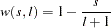
• Quadratic spectral (KERNEL=QS)

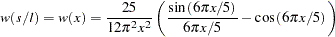
You can specify the number of lags, , in three different ways:

• Schwert (SCHW = c) (default for NW, c=4)

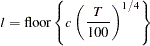
• Manual (LAG = )

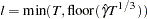
• Automatic selection (AUTO) (default for QS) Hobijn, Franses, and Ooms (2004)

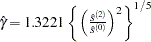
The last option (AUTO) needs more explanation, summarized in the following table.

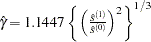
Ramsey’s Reset Test

Ramsey’s reset test is a misspecification test associated with the functional form of models to check whether power transforms need to be added to a model. The original linear model, henceforth called the restricted model, is

To test for misspecification in the functional form, the unrestricted model is

where is the predicted value from the linear model and is the power of in the unrestricted model equation starting from 2. The number of higher-ordered terms to be chosen depends on the discretion of the analyst. The RESET opti

on produces test results for 2, 3, and 4.

The reset test is an F statistic for testing , against for at least one in the unrestricted model and is computed as follows:

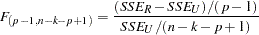where is the sum of squared errors due to the restricted model, is the sum of squared errors due to the unrestricted model, is the total number of observations, and is the number of parameters in the original linear model.

Ramsey’s test can be viewed as a linearity test that checks whether any nonlinear transformation of the specified independent variables has been omitted, but it need not help in identifying a new relevant variable other than those already specified in the current model.