| The AUTOREG Procedure |
| MODEL Statement |
- MODEL dependent = regressors / options ;
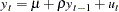
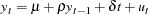
The MODEL statement specifies the dependent variable and independent regressor variables for the regression model. If no independent variables are specified in the MODEL statement, only the mean is fitted. (This is a way to obtain autocorrelations of a series.)
Models can be given labels of up to eight characters. Model labels are used in the printed output to identify the results for different models. The model label is specified as follows:
label : MODEL ...;
The following options can be used in the MODEL statement after a slash (/).
- CENTER
centers the dependent variable by subtracting its mean and suppresses the intercept parameter from the model. This option is valid only when the model does not have regressors (explanatory variables).
Autoregressive Error Options
- NLAG= number
- NLAG= ( number-list )
specifies the order of the autoregressive error process or the subset of autoregressive error lags to be fitted. Note that NLAG=3 is the same as NLAG=(1 2 3). If the NLAG= option is not specified, PROC AUTOREG does not fit an autoregressive model.
GARCH Estimation Options
- DIST= value
specifies the distribution assumed for the error term in GARCH-type estimation. If no GARCH= option is specified, the option is ignored. If EGARCH is specified, the distribution is always normal distribution. The values of the DIST= option are as follows:
- T
specifies Student’s t distribution.
- NORMAL
specifies the standard normal distribution. The default is DIST=NORMAL.
- GARCH= ( option-list )
specifies a GARCH-type conditional heteroscedasticity model. The GARCH= option in the MODEL statement specifies the family of ARCH models to be estimated. The GARCH
 regression model is specified in the following statement:
 model y = x1 x2 / garch=(q=1,p=1);
When you want to estimate the subset of ARCH terms, such as ARCH
 , you can write the SAS statement as follows:
 model y = x1 x2 / garch=(q=(1 3));
With the TYPE= option, you can specify various GARCH models. The IGARCH
 model without trend in variance is estimated as follows:
 model y = / garch=(q=2,p=1,type=integ,noint);
The following options can be used in the GARCH=( ) option. The options are listed within parentheses and separated by commas.
- Q= number
- Q= (number-list)
specifies the order of the process or the subset of ARCH terms to be fitted.
- P= number
- P= (number-list)
specifies the order of the process or the subset of GARCH terms to be fitted. If only the P= option is specified, Q=1 is assumed.
- TYPE= value
specifies the type of GARCH model. The values of the TYPE= option are as follows:
- EXP
specifies the exponential GARCH or EGARCH model.
- INTEGRATED
specifies the integrated GARCH or IGARCH model.
- NELSON | NELSONCAO
specifies the Nelson-Cao inequality constraints.
- NONNEG
specifies the GARCH model with nonnegativity constraints.
- STATIONARY
constrains the sum of GARCH coefficients to be less than 1.
The default is TYPE=NELSON.
- MEAN= value
specifies the functional form of the GARCH-M model. The values of the MEAN= option are as follows:
- LINEAR
specifies the linear function:
- LOG
specifies the log function:
- SQRT
specifies the square root function:
- NOINT
suppresses the intercept parameter in the conditional variance model. This option is valid only with the TYPE=INTEG option.
- STARTUP= MSE | ESTIMATE
requests that the positive constant c for the start-up values of the GARCH conditional error variance process be estimated. By default or if STARTUP=MSE is specified, the value of the mean squared error is used as the default constant.
- TR
uses the trust region method for GARCH estimation. This algorithm is numerically stable, though computation is expensive. The double quasi-Newton method is the default.
Printing Options
- ALL
requests all printing options.
- ARCHTEST
requests the Q and LM statistics testing for the absence of ARCH effects.
-
CHOW= ( obs
 ...obs
 )
)
computes Chow tests to evaluate the stability of the regression coefficient. The Chow test is also called the analysis-of-variance test.
Each value
 listed on the CHOW= option specifies a break point of the sample. The sample is divided into parts at the specified break point, with observations before in the first part and and later observations in the second part, and the fits of the model in the two parts are compared to whether both parts of the sample are consistent with the same model.
 The break points
refer to observations within the time range of the dependent variable, ignoring missing values before the start of the dependent series. Thus, CHOW=20 specifies the 20th observation after the first nonmissing observation for the dependent variable. For example, if the dependent variable Y contains 10 missing values before the first observation with a nonmissing Y value, then CHOW=20 actually refers to the 30th observation in the data set. When you specify the break point, you should note the number of presample missing values.
- COEF
prints the transformation coefficients for the first p observations. These coefficients are formed from a scalar multiplied by the inverse of the Cholesky root of the Toeplitz matrix of autocovariances.
- CORRB
prints the estimated correlations of the parameter estimates.
- COVB
prints the estimated covariances of the parameter estimates.
- COVEST= OP | HESSIAN | QML
specifies the type of covariance matrix for the GARCH or heteroscedasticity model. When COVEST=OP is specified, the outer product matrix is used to compute the covariance matrix of the parameter estimates. The COVEST=HESSIAN option produces the covariance matrix by using the Hessian matrix. The quasi-maximum likelihood estimates are computed with COVEST=QML. The default is COVEST=OP.
- DW= n
prints Durbin-Watson statistics up to the order n. The default is DW=1. When the LAGDEP option is specified, the Durbin-Watson statistic is not printed unless the DW= option is explicitly specified.
- DWPROB
now produces p-values for the generalized Durbin-Watson test statistics for large sample sizes. Previously, the Durbin-Watson probabilities were calculated only for small sample sizes. The new method of calculating Durbin-Watson probabilities is based on the algorithm of Ansley, Kohn, and Shively (1992).
- GINV
prints the inverse of the Toeplitz matrix of autocovariances for the Yule-Walker solution. See the section Computational Methods later in this chapter for details.
- GODFREY
- GODFREY= r
produces Godfrey’s general Lagrange multiplier test against ARMA errors.
- ITPRINT
prints the objective function and parameter estimates at each iteration. The objective function is the full log likelihood function for the maximum likelihood method, while the error sum of squares is produced as the objective function of unconditional least squares. For the ML method, the ITPRINT option prints the value of the full log likelihood function, not the concentrated likelihood.
- LAGDEP
- LAGDV
prints the Durbin t statistic, which is used to detect residual autocorrelation in the presence of lagged dependent variables. See the section Generalized Durbin-Watson Tests later in this chapter for details.
- LAGDEP= name
- LAGDV= name
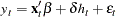
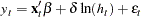
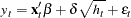
prints the Durbin h statistic for testing the presence of first-order autocorrelation when regressors contain the lagged dependent variable whose name is specified as LAGDEP=name. If the Durbin h statistic cannot be computed, the asymptotically equivalent t statistic is printed instead. See the section Generalized Durbin-Watson Tests for details.
When the regression model contains several lags of the dependent variable, specify the lagged dependent variable for the smallest lag in the LAGDEP= option. For example:
model y = x1 x2 ylag2 ylag3 / lagdep=ylag2;
- LOGLIKL
prints the log likelihood value of the regression model, assuming normally distributed errors.
- NOPRINT
- NORMAL
specifies the Jarque-Bera’s normality test statistic for regression residuals.
- PARTIAL
-
PCHOW= ( obs ...obs )
computes the predictive Chow test. The form of the PCHOW= option is the same as the CHOW= option; see the discussion of the CHOW= option earlier in this chapter.
- RESET
produces Ramsey’s RESET test statistics. The RESET option tests the null model

against the alternative
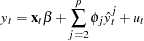
where
 is the predicted value from the OLS estimation of the null model. The RESET option produces three RESET test statistics for
  , 3, and 4.
 - STATIONARITY= ( PHILLIPS )
- STATIONARITY= ( PHILLIPS=( value ...value ) )
- STATIONARITY= ( KPSS )
- STATIONARITY= ( KPSS=(KERNEL=TYPE ) )
- STATIONARITY= ( KPSS=(KERNEL=TYPE TRUNCPOINTMETHOD) )
- STATIONARITY= ( PHILLIPS<=(...)>, KPSS<=(...)> )
specifies tests of stationarity or unit roots. The STATIONARITY= option provides Phillips-Perron, Phillips-Ouliaris, and KPSS tests.
The PHILLIPS or PHILLIPS= suboption of the STATIONARITY= option produces the Phillips-Perron unit root test when there are no regressors in the MODEL statement. When the model includes regressors, the PHILLIPS option produces the Phillips-Ouliaris cointegration test. The PHILLIPS option can be abbreviated as PP.
The PHILLIPS option performs the Phillips-Perron test for three null hypothesis cases: zero mean, single mean, and deterministic trend. For each case, the PHILLIPS option computes two test statistics,
 and
and  (in the original paper they are referred to as
  and ) , and reports their p-values. These test statistics have the same limiting distributions as the corresponding Dickey-Fuller tests.
 The three types of the Phillips-Perron unit root test reported by the PHILLIPS option are as follows.
- Zero mean
computes the Phillips-Perron test statistic based on the zero mean autoregressive model:

- Single mean
computes the Phillips-Perron test statistic based on the autoregressive model with a constant term:
- Trend
computes the Phillips-Perron test statistic based on the autoregressive model with constant and time trend terms:
You can specify several truncation points
 for weighted variance estimators by using the PHILLIPS=(
 ) specification. The statistic for each truncation point
  is computed as
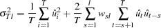
where
 and
and  are OLS residuals. If you specify the PHILLIPS option without specifying truncation points, the default truncation point is
  , where
  is the number of observations.
 The Phillips-Perron test can be used in general time series models since its limiting distribution is derived in the context of a class of weakly dependent and heterogeneously distributed data. The marginal probability for the Phillips-Perron test is computed assuming that error disturbances are normally distributed.
When there are regressors in the MODEL statement, the PHILLIPS option computes the Phillips-Ouliaris cointegration test statistic by using the least squares residuals. The normalized cointegrating vector is estimated using OLS regression. Therefore, the cointegrating vector estimates might vary with the regressand (normalized element) unless the regression R-square is 1.
The marginal probabilities for cointegration testing are not produced. You can refer to Phillips and Ouliaris (1990) tables Ia–Ic for the
 test and tables IIa–IIc for the
  test. The standard residual-based cointegration test can be obtained using the NOINT option in the MODEL statement, while the demeaned test is computed by including the intercept term. To obtain the demeaned and detrended cointegration tests, you should include the time trend variable in the regressors. Refer to Phillips and Ouliaris (1990) or Hamilton (1994, Tbl. 19.1) for information about the Phillips-Ouliaris cointegration test. Note that Hamilton (1994, Tbl. 19.1) uses
  and
and  instead of the original Phillips and Ouliaris (1990) notation. We adopt the notation introduced in Hamilton. To distinguish from Student’s
  distribu
 tion, these two statistics are named accordingly as
 (rho) and
  (tau).
 The KPSS, KPSS=(KERNEL=TYPE), or KPSS=(KERNEL=TYPE TRUNCPOINTMETHOD) specifications of the STATIONARITY= option produce the Kwiatkowski, Phillips, Schmidt, and Shin (1992) (KPSS) unit root test.
Unlike the null hypothesis of the Dickey-Fuller and Phillips-Perron tests, the null hypothesis of the KPSS states that the time series is stationary. As a result, it tends to reject a random walk more often. If the model does not have an intercept, the KPSS option performs the KPSS test for three null hypothesis cases: zero mean, single mean, and deterministic trend. Otherwise, it reports single mean and deterministic trend only. It computes a test statistic and tabulated p-values (see Hobijn, Franses, and Ooms (2004)) for the hypothesis that the random walk component of the time series is equal to zero in the following cases (for details, see Kwiatkowski, Phillips, Schmidt, and Shin (KPSS) Unit Root Test):
- Zero mean
computes the KPSS test statistic based on the zero mean autoregressive model. The p-value reported is used from Hobijn, Franses, and Ooms (2004).

- Single mean
computes the KPSS test statistic based on the autoregressive model with a constant term. The p-value reported is used from Kwiatkowski et al. (1992).

- Trend
computes the KPSS test statistic based on the autoregressive model with constant and time trend terms. The p-value reported is from Kwiatkowski et al. (1992).

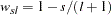
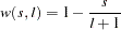
This test depends on the long-run variance of the series being defined as
where
 is a kernel,
  is a maximum lag (truncation point), and are OLS residuals or original data series. You can specify two types of the kernel:
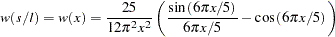
 - KERNEL=NW|BART
Newey-West (or Bartlett) kernel
- KERNEL=QS
Quadratic spectral kernel
You can set the truncation point
by using three different methods: - SCHW=c
Schwert maximum lag formula
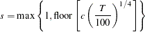
- LAG=
LAG=
manually defined number of lags. - AUTO
Automatic bandwidth selection (Hobijn, Franses, and Ooms; 2004) (for details, see Kwiatkowski, Phillips, Schmidt, and Shin (KPSS) Unit Root Test).
If STATIONARITY=KPSS is defined without additional parameters, the Newey-West kernel is used. For the Newey-West kernel the default is the Schwert truncation point method with
 . For the quadratic spectral kernel the default is AUTO.
 The KPSS test can be used in general time series models since its limiting distribution is derived in the context of a class of weakly dependent and heterogeneously distributed data. The limiting probability for the KPSS test is computed assuming that error disturbances are normally distributed.
The asymptotic distribution of the test does not depend on the presence of regressors in the MODEL statement.
The marginal probabilities for the test are reported. They are copied from Kwiatkowski et al. (1992) and Hobijn, Franses, and Ooms (2004). When there is an intercept in the model, results for mean and trend tests statistics are provided.
Examples: To test for stationarity of regression residuals, using default KERNEL= NW and SCHW= 4, you can use the following code:
   /*-- test for stationarity of regression residuals --*/
   proc autoreg data=a;
      model y=  / stationarity = (KPSS);
   run;
To test for stationarity of regression residuals, using quadratic spectral kernel and automatic bandwidth selection, you can use:
/*-- test for stationarity using quadratic spectral kernel and automatic bandwidth selection --*/ proc autoreg data=a; model y= / stationarity = (KPSS=(KERNEL=QS AUTO)); run;- URSQ
prints the uncentered regression
 . The uncentered regression is useful to compute Lagrange multiplier test statistics, since most LM test statistics are computed as T *URSQ, where T is the number of observations used in estimation.
Stepwise Selection Options
- BACKSTEP
removes insignificant autoregressive parameters. The parameters are removed in order of least significance. This backward elimination is done only once on the Yule-Walker estimates computed after the initial ordinary least squares estimation. The BACKSTEP option can be used with all estimation methods since the initial parameter values for other estimation methods are estimated using the Yule-Walker method.
Estimation Control Options
- CONVERGE= value
specifies the convergence criterion. If the maximum absolute value of the change in the autoregressive parameter estimates between iterations is less than this amount, then convergence is assumed. The default is CONVERGE=.001.
If the GARCH= option and/or the HETERO statement is specified, convergence is assumed when the absolute maximum gradient is smaller than the value specified by the CONVERGE= option or when the relative gradient is smaller than 1E–8. By default, CONVERGE=1E–5.
- INITIAL= ( initial-values )
- START= ( initial-values )
specifies initial values for some or all of the parameter estimates. The values specified are assigned to model parameters in the same order as the parameter estimates are printed in the AUTOREG procedure output. The order of values in the INITIAL= or START= option is as follows: the intercept, the regressor coefficients, the autoregressive parameters, the ARCH parameters, the GARCH parameters, the inverted degrees of freedom for Student’s t distribution, the start-up value for conditional variance, and the heteroscedasticity model parameters
 specified by the HETERO statement.
 The following is an example of specifying initial values for an AR(1)-GARCH
model with regressors X1 and X2: /*-- specifying initial values --*/ model y = w x / nlag=1 garch=(p=1,q=1) initial=(1 1 1 .5 .8 .1 .6);The model specified by this MODEL statement is


The initial values for the regression parameters, INTERCEPT (
 ), X1 (
 ), and X2 (
 ), are specified as 1. The initial value of the AR(1) coefficient (
 ) is specified as 0.5. The initial value of ARCH0 (
 ) is 0.8, the initial value of ARCH1 (
 ) is 0.1, and the initial value of GARCH1 (
 ) is 0.6.
 When you use the RESTRICT statement, the initial values specified by the INITIAL= option should satisfy the restrictions specified for the parameter estimates. If they do not, the initial values you specify are adjusted to satisfy the restrictions.
- LDW
specifies that p-values for the Durbin-Watson test be computed using a linearized approximation of the design matrix when the model is nonlinear due to the presence of an autoregressive error process. (The Durbin-Watson tests of the OLS linear regression model residuals are not affected by the LDW option.) Refer to White (1992) for Durbin-Watson testing of nonlinear models.
- MAXITER= number
sets the maximum number of iterations allowed. The default is MAXITER=50.
- METHOD= value
requests the type of estimates to be computed. The values of the METHOD= option are as follows:
- METHOD=ML
specifies maximum likelihood estimates.
- METHOD=ULS
specifies unconditional least squares estimates.
- METHOD=YW
specifies Yule-Walker estimates.
- METHOD=ITYW
specifies iterative Yule-Walker estimates.
If the GARCH= or LAGDEP option is specified, the default is METHOD=ML. Otherwise, the default is METHOD=YW.
- NOMISS
requests the estimation to the first contiguous sequence of data with no missing values. Otherwise, all complete observations are used.
- OPTMETHOD= QN | TR
specifies the optimization technique when the GARCH or heteroscedasticity model is estimated. The OPTMETHOD=QN option specifies the quasi-Newton method. The OPTMETHOD=TR option specifies the trust region method. The default is OPTMETHOD=QN.
Copyright © 2008 by SAS Institute Inc., Cary, NC, USA. All rights reserved.