Sample 64029: Area under the ROC curve measure (AUC) for multinomial models
 |  |  |  |  |
Area under the ROC curve measure (AUC) for multinomial models
| Contents: | Purpose / History / Requirements / Usage / Details / Limitations / Missing Values / See Also / References |
- PURPOSE:
- The area under the ROC curve (AUC) is a widely used measure of model performance for binary-response models such as logistic models. Hand and Till (2001) proposed an extension to this measure for responses with more than two classes. The MultAUC macro implements this extended measure.
- HISTORY:
- The version of the MultAUC macro that you are using is displayed in the log when you specify version (or any string) as the first argument. For example:
%MultAUC(version, <macro options>)The MultAUC macro always attempts to check for a later version of itself. If it is unable to do this (such as if there is no active internet connection available), the macro will issue the following message:
NOTE: Unable to check for newer versionThe computations performed by the macro are not affected by the appearance of this message.
Version Update Notes 1.3 Added prefix=. Final results data sets renamed as MultAUC and PairAUC. 1.1 Macro is now more robust to blanks and special characters in the response levels. 1.0 Initial coding - REQUIREMENTS:
- The MultAUC macro requires Base SAS® and SAS/STAT® software.
- USAGE:
- Follow the instructions in the Downloads tab of this sample to save the MultAUC macro definition. Replace the text within quotation marks in the following statement with the location of the MultAUC macro definition file on your system. In your SAS program or in the SAS editor window, specify this statement to define the MultAUC macro and make it available for use:
%inc "<location of your file containing the MultAUC macro>";
Following this statement, you can call the MultAUC macro. See the Results tab for examples.
The following macro parameters are optional:
- data=data-set-name
- Specifies the name of a data set containing a variable giving the observed response for each observation and a set of variables providing the predicted probabilities of each observation taking on each of the possible response levels. This data set is usually generated by an analytical procedure such as the LOGISTIC, GLIMMIX, DISCRIM or other procedure but could be from any source. If data= is omitted, then the last created data set is used.
The data set should contain only one observation for each original observation. Procedures that create an output data set containing multiple observations for each input observation must be edited to have only a single output observation per input observation. If the data set to be used is created by the OUTPUT statement in PROC LOGISTIC with the PREDPROBS=INDIVIDUAL option (not the PRED= option), then no alteration of the data set is needed.
- response=variable
- If specified, response= names a variable whose values identify the observed response level for each observation in the data= data set. If the data set is created by the OUTPUT statement in PROC LOGISTIC with the PREDPROBS=INDIVIDUAL option, then the response= option should be omitted. Otherwise, the values of variable must match (except possibly for a missing prefix) the names of the predicted probability variables in the data= data set. If the variable is numeric, then prefix= must also be specified to match the names of the predicted probabilities variables. If variable is a character variable, then it is recommended that any leading blanks be removed from its levels. See Limitations/Troubleshooting below for more information. The response levels (with any added prefix from prefix=) must be no more than 29 characters in length. The response= variable name should not be _from_.
- prefix=string
- Specifies a character string to add to the values in the response= variable to match the prefix string found at the beginning of the names of the predicted probability variables in the data= data set. If response= is specified and the response= variable is numeric, then prefix= is required. Do not include quotes in or around string. Use this option when the names of the predicted probability variables all begin with a character string which does not appear at the beginning of the levels of the response= variable values.
- DETAILS:
- A widely used measure of model performance for binary-response models is the area under the ROC curve (AUC) which is related to the Gini index. For a discussion of the ROC curve and the area beneath it in binary-response models, see the Receiver Operating Characteristic Curves section and the related examples in the PROC LOGISTIC chapter of the SAS/STAT User's Guide. See also Gönen (2007). For more on the ROC related capabilities in SAS, see the ROC item in the list of Frequently-Asked for Statistics.
Hand and Till (2001) extended the AUC measure to the multinomial case where the response has more than two levels. Their paper provides a good overview of both the binary and multinomial AUC statistics and their properties. Their multinomial measure reduces to the usual AUC when the response is binary (see Example 3). As with the binary AUC, the multinomial AUC ranges from 0 to 1, where 1 indicates a perfect fit and 0 represents a model that performs no better than chance. Note that in the multinomial case, a single ROC curve cannot be plotted.
The MultAUC macro is designed to work most easily with the data set created by the OUTPUT statement in PROC LOGISTIC in which the PREDPROBS=INDIVIDUAL (rather than the PRED= or P=) option is specified. When you fit a nominal (LINK=GLOGIT) or ordinal (LINK=LOGIT) model and specify the PREDPROBS=INDIVIDUAL option in the OUTPUT statement, the macro can be specified without options if called immediately after PROC LOGISTIC. If you use a different method that produces a data set with predicted probabilities of each response level for each observation, then specify response=, and prefix= if needed, to estimate the AUC.
The results from the macro are the overall AUC as well as the pairwise AUC values for each pair of response levels.
Output data sets
Results from the macro are available in two data sets. The overall AUC is saved in the MultAUC data set. The pairwise AUC values are saved in the PairAUC data set.
BY group processing
The MultAUC macro does not directly support BY group processing. That is, it cannot process results from a modeling procedure that was run using a BY statement. However, this capability can be provided by the RunBY macro which can run both the modeling procedure and the MultAUC macro for each of the BY groups in your data. See the RunBY macro documentation for details on its use. Also see the example titled "BY group processing" in the Results tab above.
- LIMITATIONS / TROUBLESHOOTING:
- No standard error, test, or confidence interval for AUC is currently available.
Some analytical procedures or methods remove leading blanks from the values of a character response variable when creating the names of the predicted probability variables. This can prevent the macro from correctly deriving the predicted probability variable names from the values of the response= variable. It is recommended that any leading blanks be removed from character response values either prior to the analysis that produces the data= data set or by modifying the values in the resulting data set. Leading (and trailing) blanks are easily removed using the CATS function in a DATA step statement such as:
response = cats(response);
- MISSING VALUES:
- Observations with missing response= variable are ignored. The variables containing the predicted probabilities for each observation must all be nonmissing. If the observation was ignored in the model fit, then all of its predicted probabilities are missing and the macro will similarly ignore the observation.
- SEE ALSO:
- "ROC" in the list of Frequently-Asked for Statistics.
- REFERENCES:
- Hand D.J. and Till R.J. (2001). "A Simple Generalisation of the Area Under the ROC Curve for Multiple Class Classification Problems." Machine Learning 45(2), p. 171-186.
These sample files and code examples are provided by SAS Institute Inc. "as is" without warranty of any kind, either express or implied, including but not limited to the implied warranties of merchantability and fitness for a particular purpose. Recipients acknowledge and agree that SAS Institute shall not be liable for any damages whatsoever arising out of their use of this material. In addition, SAS Institute will provide no support for the materials contained herein.
These sample files and code examples are provided by SAS Institute Inc. "as is" without warranty of any kind, either express or implied, including but not limited to the implied warranties of merchantability and fitness for a particular purpose. Recipients acknowledge and agree that SAS Institute shall not be liable for any damages whatsoever arising out of their use of this material. In addition, SAS Institute will provide no support for the materials contained herein.
- EXAMPLE 1: Comparing competing multinomial models using AUC
- This example uses the Iris data set that is used in examples in the PROC DISCRIM chapter and other procedure chapters in the SAS/STAT User's Guide. The Iris data set is available in the SASHELP library. Fifty specimens from each of three plant species are measured on several characteristics. In the following examples, the measurements of the sepal lengths and widths are used to classify each specimen into one of the three species. Several competing approaches are considered – multinomial logistic models (including a restricted model in PROC LOGISTIC and an unrestricted model in PROC GLIMMIX), discriminant analysis (assuming normality of the measurements and a nonparametric, nearest neighbor method), and a classification tree using PROC HPSPLIT. Additionally, an clustering method in PROC MBC is shown that ignores the species response.
The first model fit is a multinomial, generalized logit model. The EQUALSLOPES option restricts the slopes on the two logits to be equal in each of the two predictors. Since the PREDPROBS=INDIVIDUAL option is used, the MultAUC macro can be called with no options.
    proc logistic data=sashelp.iris;
      model Species = SepalLength SepalWidth / link=glogit equalslopes;
      output out=outlog predprobs=i;
      run;
    %MultAUC()
The multinomial AUC is estimated to be 0.7582. The pairwise AUCs range from chance level for the Setosa-Versicolor response pair (0.5) to near perfect for the Versicolor-Virginica pair (0.9948).

The next model is also a generalized logit model but is unrestricted, allowing for separate slopes on the two logits for both predictors. Since the output data set with predicted probabilities from GLIMMIX has multiple output observations for each input observation, it must be restructured for use in the MultAUC macro. To enable this, a variable (OBS) identifying the input observations is added to the data before analysis. PROC TRANSPOSE restructures the output data to have a single observation for each input observation. A DATA step then merges in the variable containing the observed responses. The CATS function is used just in case the response (Species) levels have leading blanks which should be removed. This data set can then be analyzed by the MultAUC macro after identifying the observed response variable.
Note that effectively the same unrestricted model can be fit in PROC LOGISTIC by simply removing the EQUALSLOPES option from the above example. However, GLIMMIX is used here to illustrate how its output data set can be modified for use with the MultAUC macro.
    data iris2;
      set sashelp.iris;
      obs=_n_;
      run;
    proc glimmix data=iris2;
      model Species = SepalLength SepalWidth  / solution dist=mult link=glogit;
      output out=outglim predicted(ilink);
      run;
    proc transpose data=outglim out=outglim2;
      by obs; id _level_; var predmu;
      run;
    data outglim3;
      merge iris2(keep=obs species) outglim2;
      by obs;
      Species=cats(Species);
      run;
    %MultAUC(response=Species)
For this model the overall and pairwise AUC values are all higher than seen for the restricted model above. The overall AUC is 0.93.
Another classification method is discriminant analysis. The following statements perform a parametric analysis that assumes that the predictors are normally distributed. The OUT= data set produced by PROC DISCRIM has the basic structure needed so no modification is needed.
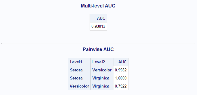
    proc discrim data=sashelp.iris out=outdis;
      class Species; var SepalLength SepalWidth;
      run;
    %MultAUC(response=Species)
The overall and pairwise AUC values for this analysis are similar to those found for the unrestricted generalized logit model above.

A nonparametric discriminant analysis is performed next using the k nearest neighbor method. For this analysis, k=9 nearest neighbors are used to develop the discriminant criterion.
    proc discrim data=sashelp.iris method=npar k=9 out=outdis;
      class Species; var SepalLength SepalWidth;
      run;
    %MultAUC(response=Species)
The overall AUC is again similar to the best results above. The AUC for the Versicolor-Virginica pair is stronger than in the previous analyses.

Next, a tree model is fit in PROC HPSPLIT using the default tree growing and pruning methods. Prior to analysis, the CATS function is used to remove any leading blanks that might exist in the response (Species) levels. Though that is not necessary in this case, it is recommended to avoid any problems that leading blanks can cause. Note that the predicted probability variable names produced by the procedure prefix the response (Species) levels with "P_Species". To match these names, prefix=p_species is specified in the MultAUC call.
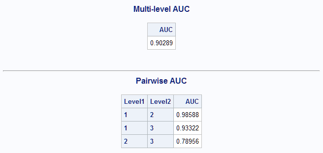
    data iris; set sashelp.iris;
      Species=cats(Species);
      run;
    proc hpsplit data=iris seed=48393;
      class Species;
      model Species = SepalLength SepalWidth;
      output out=outspt;
      run;
    %MultAUC(response=Species, prefix=p_species)
The overall AUC (0.90) is not quite as good as some of the models above.

The above modeling methods are known as supervised methods since the response is known and is used in developing the model. There are also unsupervised methods, such as clustering methods, that can be used to find groups in data when the true classifications of the observations are not known. Observations that are similar, based on some criterion, are grouped together in a cluster. SAS/STAT procedures that implement such clustering methods include the CLUSTER, FASTCLUS, and MODECLUS procedures. Model-based clustering is also available beginning in SAS® Viya® 3.4 and is used next.
Since this is an unsupervised method, the true classifications in the Species variable are not used. The method finds clusters of the observations based on their similarity using only the SepalLength and SepalWidth measurements. After creating a CAS table of the Iris data, the following statements initialize the method using k-means clustering and request a three-cluster solution. All possible covariance structures, as specified in the CONSTRUCT= option, are considered in choosing a final model. The output data set contains the cluster membership from the model for each observation (MAXPOST) and the posterior probabilities of membership in each cluster (named NEXT1, NEXT2, and NEXT3, where 1, 2, and 3 refer to the cluster number). The COPYVARS= option copies the Species, SepalLength, and SepalWidth variables from the input data set.
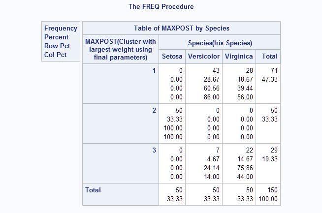
    proc mbc data=casuser.iris nclusters=(3) init=kmeans seed=1418410433
             covstruct=(EEE EEI EEV EII EVI EVV VII VVI VVV);
      var SepalLength SepalWidth;
      output out=casuser.scores maxpost copyvars=(Species SepalLength SepalWidth);
      run;
The following produces a cross-classification of the cluster numbers assigned to the observations and the known Species levels.
    proc freq data=casuser.scores;
      table maxpost*Species;
      run;
Notice that cluster 2 exactly contains the Setosa observations. While clusters 1 and 3 do not completely separate the other two Species, cluster 1 contains mostly Versicolor observations and cluster 3 mostly Virginica observations.
These statements name the cluster posterior probability variables according to the Species with which they correspond as shown above, and then call the MultAUC macro.
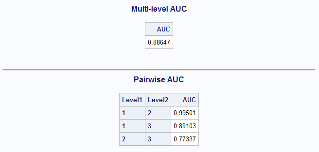
    data casuser.scores;
      set casuser.scores;
      Setosa     = next2;
      Virginica  = next3;
      Versicolor = next1;
      run;
    %MultAUC(data=casuser.scores, response=Species)
The resulting AUC (0.92) is only slightly below the best models above.

Among the models and methods considered above, the best performing models as judged by the AUC are the unrestricted generalized logit model and the nonparametric discriminant model with AUC values approximately equal to 0.93. Of course, all of these models and methods of estimating them could be altered in various ways, so it is possible that better models of each type could be found.
- EXAMPLE 2: Computing AUC for a test data set
- This example uses the wine data from the Getting Started section in the PROC HPSPLIT chapter of the SAS/STAT User's Guide. The data record a three-level variable, Cultivar, and 13 chemical attributes on 178 wine samples. The following statements creates a random 60% training subset and 40% test subset of the data. Computing the AUC on the data used to train a model can result in an overly optimistic value. By using a test data set for the computation, a more realistic AUC estimate can be obtained.
    data Winetrn Winetst;
      set Wine;
      if ranuni(8473)>=.4 then output Winetrn;
      else output Winetst;
      run;
The LASSO selection method in PROC HPGENSELECT can be used to select the important predictors to use in a model. The following identifies Mg and Proline as the final model from the LASSO method.
    proc hpgenselect data=Winetrn;
      model Cultivar = Alcohol Malic Ash Alkan Mg TotPhen Flav
                       NFPhen Cyanins Color Hue ODRatio Proline
                       / dist=mult link=glogit;
      selection method=lasso;
      run;
The selected model is fit in PROC LOGISTIC and the test data set is scored by the SCORE statement using the fitted model. The training data set is also scored by the OUTPUT data set.
    proc logistic data=Winetrn;
      model Cultivar = Mg Proline / link=glogit;
      score data=Winetst out=Winetst;
      output out=Predtrn predprobs=i;
      run;
The MultAUC macro can be called to compute the AUC for each of the training and test data sets. The predicted probability variable names in the OUT= data set created by the SCORE statement use the prefix P_. The data set also contains the character variable, F_Cultivar, which contains the observed response levels. Specifying prefix=P_ adds the prefix to the response levels to match the predicted probability variable names.
    %MultAUC(data=Predtrn)
    %MultAUC(data=Winetst, response=F_Cultivar. prefix=P_)
Using the LASSO-selected model developed above, the estimated AUC for the training data set is 0.90.
For the test data set, the selected model estimates the AUC as 0.89 which is slightly less optimistic than was obtained above from the training data set.
- EXAMPLE 3: AUC for binary response model
- This example uses the cancer remission data from the example titled "Stepwise Logistic Regression and Predicted Values" in the PROC LOGISTIC chapter of the SAS/STAT User's Guide. The multinomial AUC proposed by Hand and Till (2001) reduces to the usual AUC when the response is binary. To illustrate this, the following PROC LOGISTIC statements fit a model to the binary response, Remiss, and compute the usual AUC. The predicted probabilities are saved by the PREDPROBS=INDIVIDUAL option in the OUTPUT statement.
    proc logistic data=Remission;
      model remiss(event="1")=blast;
      output out=out predprobs=i;
      run;
The AUC is presented as the c statistic in the "Association of Predicted Probabilities and Observed Responses" table and is estimated as 0.753.

Next, the multinomial AUC is computed by the MultAUC macro.
%MultAUC()The same value results from the computation of the multinomial AUC.

- EXAMPLE 4: BY group processing
- The MultAUC macro cannot process results from a modeling procedure that used a BY statement. However, the RunBY macro can be used to run both the modeling procedure and the MultAUC macro on BY groups in the data. The following uses the data in Long (1997) that has a four-point ordinal response (WARM) concerning the warmth of a working mother's relationship to her child. The AUC is to be estimated by child's gender (MALE) using separate models fit to the data for each gender.
In the statements below, a WHERE statement is included in the LOGISTIC modeling step to subset the input data to one level of MALE. The special macro variables, _BYx and _LVLx, are used by the RunBY macro to fit the model to each BY group and then to run the MultAUC macro. The BYlabel macro variable is specified in a TITLE statement in LOGISTIC and in a FOOTNOTE statement prior to the MultAUC call to label the displayed results with the BY group definition.
      %macro code();
         proc logistic data=LongData;
            where &_BY1=&_LVL1;
            model warm(desc)=yr89 white age ed prst;
            output out=outlog predprobs=i;
            title "&BYlabel";
            run;
         footnote "Above for &BYlabel";
         %MultAUC();
         footnote;
      %mend;
      %RunBY(data=LongData, by=male)
Right-click on the link below and select Save to save the MultAUC macro definition to a file. It is recommended that you name the file MultAUC.sas.
| Type: | Sample |
| Topic: | Analytics ==> Categorical Data Analysis Analytics ==> Regression SAS Reference ==> Procedures ==> DISCRIM SAS Reference ==> Procedures ==> GENMOD SAS Reference ==> Procedures ==> GLIMMIX SAS Reference ==> Procedures ==> HPGENSELECT SAS Reference ==> Procedures ==> HPSPLIT SAS Reference ==> Procedures ==> LOGISTIC |
| Date Modified: | 2020-07-28 16:24:33 |
| Date Created: | 2019-04-11 15:46:21 |
Operating System and Release Information
| Product Family | Product | Host | SAS Release | |
| Starting | Ending | |||
| SAS System | SAS/STAT | z/OS | ||
| z/OS 64-bit | ||||
| OpenVMS VAX | ||||
| Microsoft® Windows® for 64-Bit Itanium-based Systems | ||||
| Microsoft Windows Server 2003 Datacenter 64-bit Edition | ||||
| Microsoft Windows Server 2003 Enterprise 64-bit Edition | ||||
| Microsoft Windows XP 64-bit Edition | ||||
| Microsoft® Windows® for x64 | ||||
| OS/2 | ||||
| Microsoft Windows 8 Enterprise 32-bit | ||||
| Microsoft Windows 8 Enterprise x64 | ||||
| Microsoft Windows 8 Pro 32-bit | ||||
| Microsoft Windows 8 Pro x64 | ||||
| Microsoft Windows 8.1 Enterprise 32-bit | ||||
| Microsoft Windows 8.1 Enterprise x64 | ||||
| Microsoft Windows 8.1 Pro 32-bit | ||||
| Microsoft Windows 8.1 Pro x64 | ||||
| Microsoft Windows 10 | ||||
| Microsoft Windows 95/98 | ||||
| Microsoft Windows 2000 Advanced Server | ||||
| Microsoft Windows 2000 Datacenter Server | ||||
| Microsoft Windows 2000 Server | ||||
| Microsoft Windows 2000 Professional | ||||
| Microsoft Windows NT Workstation | ||||
| Microsoft Windows Server 2003 Datacenter Edition | ||||
| Microsoft Windows Server 2003 Enterprise Edition | ||||
| Microsoft Windows Server 2003 Standard Edition | ||||
| Microsoft Windows Server 2003 for x64 | ||||
| Microsoft Windows Server 2008 | ||||
| Microsoft Windows Server 2008 R2 | ||||
| Microsoft Windows Server 2008 for x64 | ||||
| Microsoft Windows Server 2012 Datacenter | ||||
| Microsoft Windows Server 2012 R2 Datacenter | ||||
| Microsoft Windows Server 2012 R2 Std | ||||
| Microsoft Windows Server 2012 Std | ||||
| Microsoft Windows Server 2016 | ||||
| Microsoft Windows Server 2019 | ||||
| Microsoft Windows XP Professional | ||||
| Windows 7 Enterprise 32 bit | ||||
| Windows 7 Enterprise x64 | ||||
| Windows 7 Home Premium 32 bit | ||||
| Windows 7 Home Premium x64 | ||||
| Windows 7 Professional 32 bit | ||||
| Windows 7 Professional x64 | ||||
| Windows 7 Ultimate 32 bit | ||||
| Windows 7 Ultimate x64 | ||||
| Windows Millennium Edition (Me) | ||||
| Windows Vista | ||||
| Windows Vista for x64 | ||||
| 64-bit Enabled AIX | ||||
| 64-bit Enabled HP-UX | ||||
| 64-bit Enabled Solaris | ||||
| ABI+ for Intel Architecture | ||||
| AIX | ||||
| HP-UX | ||||
| HP-UX IPF | ||||
| IRIX | ||||
| Linux | ||||
| Linux for x64 | ||||
| Linux on Itanium | ||||
| OpenVMS Alpha | ||||
| OpenVMS on HP Integrity | ||||
| Solaris | ||||
| Solaris for x64 | ||||
| Tru64 UNIX | ||||