The SURVEYMEANS Procedure

Statistical Computations
- Definitions and Notation
- Mean
- Variance and Standard Error of the Mean
- t Test for the Mean
- Degrees of Freedom
- Confidence Limits for the Mean
- Coefficient of Variation
- Proportions
- Total
- Variance and Standard Deviation of the Total
- Confidence Limits for the Total
- Ratio
- Domain Statistics
- Quantiles
- Geometric Mean
- Poststratification
The SURVEYMEANS procedure uses the Taylor series (linearization) method or replication (resampling) methods to estimate sampling errors of estimators based on complex sample designs. For more information, see Fuller (2009); Wolter (2007); Lohr (2010); Kalton (1983); Hidiroglou, Fuller, and Hickman (1980); Fuller et al. (1989); Lee, Forthofer, and Lorimor (1989); Cochran (1977); Kish (1965); Hansen, Hurwitz, and Madow (1953); Rust (1985); Dippo, Fay, and Morganstein (1984); Rao and Shao (1999); Rao, Wu, and Yue (1992); Rao and Shao (1996). You can use the VARMETHOD= option to specify a variance estimation method to use. By default, the Taylor series method is used.
The Taylor series method obtains a linear approximation for the estimator and then uses the variance estimate for this approximation to estimate the variance of the estimate itself (Woodruff 1971; Fuller 1975). When there are clusters, or PSUs, in the sample design, the procedure estimates variance from the variation among PSUs. When the design is stratified, the procedure pools stratum variance estimates to compute the overall variance estimate. For t tests of the estimates, the degrees of freedom equal the number of clusters minus the number of strata in the sample design.
For a multistage sample design, the Taylor series estimation depends only on the first stage of the sample design. Therefore, the required input includes only first-stage cluster (PSU) and first-stage stratum identification. You do not need to input design information about any additional stages of sampling. This variance estimation method assumes that the first-stage sampling fraction is small, or that the first-stage sample is drawn with replacement, as it often is in practice.
Quite often in complex surveys, respondents have unequal weights, which reflect unequal selection probabilities and adjustments for nonresponse. In such surveys, the appropriate sampling weights must be used to obtain valid estimates for the study population.
However, replication methods have recently gained popularity for estimating variances in complex survey data analysis. One reason for this popularity is the relative simplicity of replication-based estimates, especially for nonlinear estimators; another is that modern computational capacity has made replication methods feasible for practical survey analysis.
Replication methods draw multiple replicates (also called subsamples) from a full sample according to a specific resampling scheme. The most commonly used resampling schemes are the balanced repeated replication (BRR) method and the jackknife method. For each replicate, the original weights are modified for the PSUs in the replicates to create replicate weights. The population parameters of interest are estimated by using the replicate weights for each replicate. Then the variances of parameters of interest are estimated by the variability among the estimates derived from these replicates. You can use a REPWEIGHTS statement to provide your own replicate weights for variance estimation. For more information about using replication methods to analyze sample survey data, see the section Replication Methods for Variance Estimation.
Definitions and Notation
For a stratified clustered sample design, together with the sampling weights, the sample can be represented by an  matrix
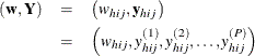
where
-
 is the stratum index
-
 is the cluster index within stratum h
-
 is the unit index within cluster i of stratum h
-
 is the analysis variable number, with a total of P variables
-
 is the total number of observations in the sample
-
 denotes the sampling weight for unit j in cluster i of stratum h
-
 are the observed values of the analysis variables for unit j in cluster i of stratum h, including both the values of numerical variables and the values of indicator variables for levels of categorical variables.
For a categorical variable
C, let l denote the number of levels of C, and denote the level values as  . Let
. Let 
 be an indicator variable for the category
 with the observed value in unit j in cluster i of stratum h:
![\[ y_{hij}^{(q)} = I_{\{ C=c_ k\} }(h,i,j) = \left\{ \begin{array}{ll} 1 & \mbox{if } C_{hij}=c_ k \\ 0 & \mbox{otherwise} \end{array} \right. \]](images/statug_surveymeans0035.png)
Note that the indicator variable  is set to missing when
  is missing. Therefore, the total number of analysis variables, P, is the total number of numerical variables plus the total number of levels of all categorical variables.
The sampling rate  for stratum h, which is used in Taylor series variance estimation, is the fraction of first-stage units (PSUs) selected for the sample.
You can use the TOTAL= or RATE= option to input population totals or sampling rates. See the section Specification of Population Totals and Sampling Rates for details. If you input stratum totals, PROC SURVEYMEANS computes as the ratio of the stratum sample size to the stratum total. If you input stratum sampling rates, PROC SURVEYMEANS uses
these values directly for . If you do not specify the TOTAL= or RATE= option, then the procedure assumes that the stratum sampling rates are negligible, and a finite population correction is not used when computing variances. Replication methods specified by
the VARMETHOD=BRR
or the VARMETHOD=JACKKNIFE
option do not use this finite population correction .
for stratum h, which is used in Taylor series variance estimation, is the fraction of first-stage units (PSUs) selected for the sample.
You can use the TOTAL= or RATE= option to input population totals or sampling rates. See the section Specification of Population Totals and Sampling Rates for details. If you input stratum totals, PROC SURVEYMEANS computes as the ratio of the stratum sample size to the stratum total. If you input stratum sampling rates, PROC SURVEYMEANS uses
these values directly for . If you do not specify the TOTAL= or RATE= option, then the procedure assumes that the stratum sampling rates are negligible, and a finite population correction is not used when computing variances. Replication methods specified by
the VARMETHOD=BRR
or the VARMETHOD=JACKKNIFE
option do not use this finite population correction .
Mean
When you specify the keyword MEAN, the procedure computes the estimate of the mean (mean per element) from the survey data. Also, the procedure computes the mean by default if you do not specify any statistic-keywords in the PROC SURVEYMEANS statement.
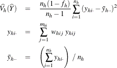
PROC SURVEYMEANS computes the estimate of the mean as
![\[ \widehat{\bar{Y}} = \left( \sum _{h=1}^ H\sum _{i=1}^{n_ h} \sum _{j=1}^{m_{hi}} ~ w_{hij} ~ y_{hij} \right) / ~ w_{\cdot \cdot \cdot } \]](images/statug_surveymeans0039.png)
where
![\[ w_{\cdot \cdot \cdot } = \sum _{h=1}^ H\sum _{i=1}^{n_ h} \sum _{j=1}^{m_{hi}} w_{hij} \]](images/statug_surveymeans0040.png)
is the sum of the weights over all observations in the sample.
Variance and Standard Error of the Mean
When you specify the keyword STDERR, the procedure computes the standard error of the mean. Also, the procedure computes the standard error by default if you specify the keyword MEAN, or if you do not specify any statistic-keywords in the PROC SURVEYMEANS statement. The keyword VAR requests the variance of the mean.
Taylor Series Method
When you use VARMETHOD=TAYLOR
, or by default if you do not specify the VARMETHOD= option, PROC SURVEYMEANS uses the Taylor series method to estimate the
variance of the mean  . The procedure computes the estimated variance as
![\[ \widehat{V}(\widehat{\bar{Y}}) = \sum _{h=1}^ H { \widehat{V_ h}(\widehat{\bar{Y}})} \]](images/statug_surveymeans0042.png)
where, if  , then
and if  , then
![\[ \widehat{V_ h}(\widehat{\bar{Y}}) = \left\{ \begin{array}{ll} \mbox{missing} & \mbox{ if } n_{h'}=1 \mbox{ for } h’=1, 2, \ldots , H \\ 0 & \mbox{ if } n_{h'}>1 \mbox{ for some } 1 \le h’ \le H \end{array} \right. \]](images/statug_surveymeans0046.png)
Replication Methods
When you specify VARMETHOD=BRR
or VARMETHOD=JACKKNIFE
, the procedure computes the variance  with replication methods by using the variability among replicate estimates to estimate the overall variance. See the section
Replication Methods for Variance Estimation for more details.
with replication methods by using the variability among replicate estimates to estimate the overall variance. See the section
Replication Methods for Variance Estimation for more details.
Standard Error
The standard error of the mean is the square root of the estimated variance.
![\[ \mbox{StdErr}(\widehat{{\bar{Y}}})= \sqrt {\widehat{V}(\widehat{\bar{Y}})} \]](images/statug_surveymeans0048.png)
t Test for the Mean
If you specify the keyword T, PROC SURVEYMEANS computes the t-value for testing that the population mean equals zero,  . The test statistic equals
![\[ t(\widehat{{\bar{Y}}}) = {\widehat{{\bar{Y}}}} ~ / ~ {\mbox{StdErr}(\widehat{{\bar{Y}}})} \]](images/statug_surveymeans0050.png)
The two-sided p-value for this test is
![\[ \mbox{Prob}(~ |T|>|t(\widehat{{\bar{Y}}})|~ ) \]](images/statug_surveymeans0051.png)
where T is a random variable with the t distribution with df degrees of freedom.
Degrees of Freedom
PROC SURVEYMEANS computes degrees of freedom df to obtain the  % confidence limits for means, proportions, totals, ratios, and other statistics. The degrees of freedom computation depends
on the variance estimation method that you request. Missing values can affect the degrees of freedom computation. See the
section Missing Values for details.
% confidence limits for means, proportions, totals, ratios, and other statistics. The degrees of freedom computation depends
on the variance estimation method that you request. Missing values can affect the degrees of freedom computation. See the
section Missing Values for details.
Taylor Series Variance Estimation
For the Taylor series method, PROC SURVEYMEANS calculates the degrees of freedom for the t test as the number of clusters minus the number of strata. If there are no clusters, then the degrees of freedom equal the number of observations minus the number of strata. If the design is not stratified, then the degrees of freedom equal the number of PSUs minus one.
If all observations in a stratum are excluded from the analysis due to missing values, then that stratum is called an empty stratum. Empty strata are not counted in the total number of strata for the table. Similarly, empty clusters and missing observations are not included in the total counts of cluster and observations that are used to compute the degrees of freedom for the analysis.
If you specify the MISSING option, missing values are treated as valid nonmissing levels for a categorical variable and are included in computing degrees of freedom. If you specify the NOMCAR option for Taylor series variance estimation, observations with missing values for an analysis variable are included in computing degrees of freedom.
Replicate-Based Variance Estimation
When there is a REPWEIGHTS statement, the degrees of freedom equal the number of REPWEIGHTS variables, unless you specify an alternative in the DF= option in a REPWEIGHTS statement.
For BRR or jackknife variance estimation without a REPWEIGHT statement, by default PROC SURVEYMEANS computes the degrees of freedom by using all valid observations in the input data set. A valid observation is an observation that has a positive value of the WEIGHT variable and nonmissing values of the STRATA and CLUSTER variables unless you specify the MISSING option. See the section Data and Sample Design Summary for details about valid observations.
For BRR variance estimation (including Fay’s method ) without a REPWEIGHTS statement, PROC SURVEYMEANS calculates the degrees of freedom as the number of strata. PROC SURVEYMEANS bases the number of strata on all valid observations in the data set, unless you specify the DFADJ method-option for VARMETHOD=BRR . When you specify the DFADJ option, the procedure computes the degrees of freedom as the number of nonmissing strata for an analysis variable. This excludes any empty strata that occur when observations with missing values of that analysis variable are removed.
For jackknife variance estimation without a REPWEIGHTS statement, PROC SURVEYMEANS calculates the degrees of freedom as the number of clusters (or number of observations if there are no clusters) minus the number of strata (or one if there are no strata). For jackknife variance estimation, PROC SURVEYMEANS bases the number of strata and clusters on all valid observations in the data set, unless you specify the DFADJ method-option for VARMETHOD=JACKKNIFE . When you specify the DFADJ option, the procedure computes the degrees of freedom from the number of nonmissing strata and clusters for an analysis variable. This excludes any empty strata or clusters that occur when observations with missing values of an analysis variable are removed.
The procedure displays the degrees of freedom for the t test if you specify the keyword DF in the PROC SURVEYMEANS statement.
Confidence Limits for the Mean
If you specify the keyword CLM, the procedure computes two-sided confidence limits for the mean. Also, the procedure includes the confidence limits by default if you do not specify any statistic-keywords in the PROC SURVEYMEANS statement.
The confidence coefficient is determined by the value of the ALPHA= option, which by default equals 0.05 and produces 95% confidence limits. The confidence limits are computed as
![\[ \widehat{\bar{Y}} \pm \mbox{StdErr}(\widehat{{\bar{Y}}})~ t_{\mi{df},\, \, \alpha /2} \]](images/statug_surveymeans0052.png)
where is the estimate of the mean,  is the standard error of the mean, and
  is the
  th percentile of the t distribution with df calculated as in the section t Test for the Mean.
If you specify the keyword UCLM, the procedure computes the one-sided upper  % confidence limit for the mean:
![\[ \widehat{\bar{Y}} + \mbox{StdErr}(\widehat{{\bar{Y}}})~ t_{\mi{df},\, \, \alpha } \]](images/statug_surveymeans0057.png)
If you specify the keyword LCLM, the procedure computes the one-sided lower % confidence limit for the mean:
![\[ \widehat{\bar{Y}} - \mbox{StdErr}(\widehat{{\bar{Y}}})~ t_{\mi{df},\, \, \alpha } \]](images/statug_surveymeans0058.png)
Coefficient of Variation
If you specify the keyword CV, PROC SURVEYMEANS computes the coefficient of variation, which is the ratio of the standard error of the mean to the estimated mean:
![\[ \mr{cv}(\bar{Y}) = \mbox{StdErr}(\widehat{{\bar{Y}}}) ~ /~ \widehat{{\bar{Y}}} \]](images/statug_surveymeans0059.png)
If you specify the keyword CVSUM, PROC SURVEYMEANS computes the coefficient of variation for the estimated total, which is the ratio of the standard deviation of the sum to the estimated total:
![\[ \mr{cv}(Y) = \mbox{Std}(\widehat{Y}) ~ /~ \widehat{Y} \]](images/statug_surveymeans0060.png)
Proportions
If you specify the keyword MEAN for a categorical variable, PROC SURVEYMEANS estimates the proportion, or relative frequency, for each level of the categorical variable. If you do not specify any statistic-keywords in the PROC SURVEYMEANS statement, the procedure estimates the proportions for levels of the categorical variables, together with their standard errors and confidence limits.
The procedure estimates the proportion in level  for variable C as
![\[ \hat p=\frac{\sum _{h=1}^ H\sum _{i=1}^{n_ h} \sum _{j=1}^{m_{hi}} ~ w_{hij} ~ y_{hij}^{(q)}}{\sum _{h=1}^ H\sum _{i=1}^{n_ h} \sum _{j=1}^{m_{hi}} ~ w_{hij}} \]](images/statug_surveymeans0062.png)
where  is the value of the indicator function for level , defined in the section Definitions and Notation, and equals 1 if the observed value of variable C equals , and equals 0 otherwise. Since the proportion estimator is actually an estimator of the mean for an indicator variable, the procedure
computes its variance and standard error according to the method outlined in the section Variance and Standard Error of the Mean. Similarly, the procedure computes confidence limits for proportions as in the section Confidence Limits for the Mean.
is the value of the indicator function for level , defined in the section Definitions and Notation, and equals 1 if the observed value of variable C equals , and equals 0 otherwise. Since the proportion estimator is actually an estimator of the mean for an indicator variable, the procedure
computes its variance and standard error according to the method outlined in the section Variance and Standard Error of the Mean. Similarly, the procedure computes confidence limits for proportions as in the section Confidence Limits for the Mean.
Total
If you specify the keyword SUM, the procedure computes the estimate of the population total from the survey data. The estimate of the total is the weighted sum over the sample:
![\[ \widehat{Y} = \sum _{h=1}^ H\sum _{i=1}^{n_ h} \sum _{j=1}^{m_{hi}} ~ w_{hij} ~ y_{hij} \]](images/statug_surveymeans0064.png)
For a categorical variable level,  estimates its total frequency in the population.
Variance and Standard Deviation of the Total
When you specify the keyword STD or the keyword SUM, the procedure estimates the standard deviation of the total. The keyword VARSUM requests the variance of the total.
Taylor Series Method
When you use VARMETHOD=TAYLOR , or by default, PROC SURVEYMEANS uses the Taylor series method to estimate the variance of the total as
![\[ \widehat{V}(\widehat{Y}) = \sum _{h=1}^ H \widehat{V_ h}(\widehat{Y}) \]](images/statug_surveymeans0066.png)
where, if , then
and if , then
![\[ \widehat{V_ h}(\widehat{Y}) = \left\{ \begin{array}{ll} \mbox{missing} & \mbox{ if } n_{h'}=1 \mbox{ for } h’=1, 2, \ldots , H \\ 0 & \mbox{ if } n_{h'}>1 \mbox{ for some } 1 \le h’ \le H \end{array} \right. \]](images/statug_surveymeans0068.png)
Replication Methods
When you specify VARMETHOD=BRR
or VARMETHOD=JACKKNIFE
option, the procedure computes the variance  with replication methods by measuring the variability among the estimates derived from these replicates. See the section
Replication Methods for Variance Estimation for more details.
with replication methods by measuring the variability among the estimates derived from these replicates. See the section
Replication Methods for Variance Estimation for more details.
Standard Deviation
The standard deviation of the total equals
![\[ \mbox{Std}(\widehat{Y})= \sqrt {\widehat{V}(\widehat{Y})} \]](images/statug_surveymeans0070.png)
Confidence Limits for the Total
If you specify the keyword CLSUM, the procedure computes confidence limits for the total. The confidence coefficient is determined by the value of the ALPHA= option, which by default equals 0.05 and produces 95% confidence limits. The confidence limits are computed as
![\[ \widehat{Y} \pm \mbox{Std}(\widehat{Y})~ t_{\mi{df},\, \, \alpha /2} \]](images/statug_surveymeans0071.png)
where  is the estimate of the total,
  is the estimated standard deviation, and is the th percentile of the t distribution with df calculated as described in the section t Test for the Mean.
If you specify the keyword UCLSUM, the procedure computes the one-sided upper % confidence limit for the sum:
![\[ \widehat{Y} + \mbox{Std}(\widehat{Y})~ t_{\mi{df},\, \, \alpha } \]](images/statug_surveymeans0074.png)
If you specify the keyword LCLSUM, the procedure computes the one-sided lower % confidence limit for the sum:
![\[ \widehat{Y} - \mbox{Std}(\widehat{Y})~ t_{\mi{df},\, \, \alpha } \]](images/statug_surveymeans0075.png)
Ratio
When you use a RATIO statement, the procedure produces statistics requested by the statistic-keywords in the PROC SURVEYMEANS statement.
Suppose that you want to calculate the ratio of variable Y to variable X. Let  be the value of variable X for the jth member in cluster i in the hth stratum.
The ratio of Y to X is
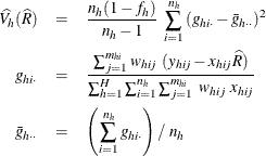
![\[ \widehat{R} = \frac{ \sum _{h=1}^ H\sum _{i=1}^{n_ h} \sum _{j=1}^{m_{hi}} ~ w_{hij} ~ y_{hij} }{ \sum _{h=1}^ H\sum _{i=1}^{n_ h} \sum _{j=1}^{m_{hi}} ~ w_{hij} ~ x_{hij} } \]](images/statug_surveymeans0077.png)
PROC SURVEYMEANS uses the Taylor series method to estimate the variance of the ratio  as
as
![\[ \widehat{V}(\widehat{R}) = \sum _{h=1}^ H \widehat{V_ h}(\widehat{R}) \]](images/statug_surveymeans0079.png)
where, if , then
and if , then
![\[ \widehat{V_ h}(\widehat{R}) = \left\{ \begin{array}{ll} \mbox{missing} & \mbox{ if } n_{h'}=1 \mbox{ for } h’=1, 2, \ldots , H \\ 0 & \mbox{ if } n_{h'}>1 \mbox{ for some } 1 \le h’ \le H \end{array} \right. \]](images/statug_surveymeans0081.png)
The standard error of the ratio is the square root of the estimated variance:
![\[ \mbox{StdErr}(\widehat{R})= \sqrt {\widehat{V}(\widehat{R})} \]](images/statug_surveymeans0082.png)
When the denominator for a ratio is zero, then the value of the ratio is displayed as '–Infty', 'Infty', or a missing value, depending on whether the numerator is negative, positive, or zero, respectively; and the corresponding internal value is the special missing value '.M', the special missing value '.I', or the usual missing value, respectively.
Domain Statistics
When you use a DOMAIN statement to request a domain analysis, the procedure computes the requested statistics for each domain.
For a domain D, let  be the corresponding indicator variable:
![\[ I_{D}(h,i,j) = \left\{ \begin{array}{ll} 1 & \mbox{if observation }(h,i,j)\mbox{ belongs to } D \\ 0 & \mbox{otherwise} \end{array} \right. \]](images/statug_surveymeans0084.png)
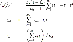
Let
![\[ z_{hij}\hspace{.1in}=\hspace{.1in} y_{hij}I_ D(h,i,j) \hspace{.1in} = \left\{ \begin{array}{ll} y_{hij} & \mbox{if observation }(h,i,j)\mbox{ belongs to } D \\ 0 & \mbox{otherwise} \end{array} \right. \]](images/statug_surveymeans0085.png)
Let
![\[ v_{hij}= w_{hij}I_ D(h,i,j) = \left\{ \begin{array}{ll} w_{hij} & \mbox{if observation }(h,i,j) \mbox{belongs to} D \\ 0 & \mbox{otherwise} \end{array} \right. \]](images/statug_surveymeans0086.png)
The requested statistics for variable y in domain D are computed by using the new weights v.
Note that  is set to missing if
  represents a level of a categorical variable and is missing.
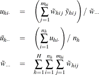
Domain Mean
The estimated mean of y in the domain D is
![\[ \widehat{\bar{Y}_ D} = \left( \sum _{h=1}^ H\sum _{i=1}^{n_ h} \sum _{j=1}^{m_{hi}} ~ v_{hij} ~ y_{hij} \right) / ~ v_{\cdot \cdot \cdot } \]](images/statug_surveymeans0089.png)
where
![\[ v_{\cdot \cdot \cdot } = \sum _{h=1}^ H\sum _{i=1}^{n_ h} \sum _{j=1}^{m_{hi}} v_{hij} \]](images/statug_surveymeans0090.png)
The variance of  is estimated by
![\[ \widehat{V}(\widehat{\bar{Y}_ D}) = \sum _{h=1}^ H \widehat{V_ h}(\widehat{\bar{Y}_ D}) \]](images/statug_surveymeans0092.png)
where, if , then
and if , then
![\[ \widehat{V_ h}(\widehat{\bar{Y}_ D}) = \left\{ \begin{array}{ll} \mbox{missing} & \mbox{ if } n_{h'}=1 \mbox{ for } h’=1, 2, \ldots , H \\ 0 & \mbox{ if } n_{h'}>1 \mbox{ for some } 1 \le h’ \le H \end{array} \right. \]](images/statug_surveymeans0094.png)
Domain Total
The estimated total in domain D is
![\[ \widehat{Y}_ D = \sum _{h=1}^ H\sum _{i=1}^{n_ h} \sum _{j=1}^{m_{hi}} ~ v_{hij} ~ y_{hij} \]](images/statug_surveymeans0095.png)
and its estimated variance is
![\[ \widehat{V}(\widehat{Y}_ D) = \sum _{h=1}^ H \widehat{V_ h}(\widehat{Y}_ D) \]](images/statug_surveymeans0096.png)
where, if , then
and if , then
![\[ \widehat{V_ h}(\widehat{Y}_ D) = \left\{ \begin{array}{ll} \mbox{missing} & \mbox{ if } n_{h'}=1 \mbox{ for } h’=1, 2, \ldots , H \\ 0 & \mbox{ if } n_{h'}>1 \mbox{ for some } 1 \le h’ \le H \end{array} \right. \]](images/statug_surveymeans0098.png)
Domain Ratio
The estimated ratio of Y to X in domain D is
![\[ \widehat{R}_ D = \frac{ \sum _{h=1}^ H\sum _{i=1}^{n_ h} \sum _{j=1}^{m_{hi}} ~ v_{hij} ~ y_{hij} }{ \sum _{h=1}^ H\sum _{i=1}^{n_ h} \sum _{j=1}^{m_{hi}} ~ v_{hij} ~ x_{hij} } \]](images/statug_surveymeans0099.png)
and its estimated variance is
![\[ \widehat{V}(\widehat{R}_ D) = \sum _{h=1}^ H \widehat{V_ h}(\widehat{R}_ D) \]](images/statug_surveymeans0100.png)
where, if , then
and if , then
![\[ \widehat{V_ h}(\widehat{R}_ D) = \left\{ \begin{array}{ll} \mbox{missing} & \mbox{ if } n_{h'}=1 \mbox{ for } h’=1, 2, \ldots , H \\ 0 & \mbox{ if } n_{h'}>1 \mbox{ for some } 1 \le h’ \le H \end{array} \right. \]](images/statug_surveymeans0102.png)
For domain analysis with poststratification, see the section Poststratification. For quantile estimation in a domain, see the section Domain Quantile. For quantile estimation in a domain with poststratification, see the section Domain Quantile Estimation with Poststratification.
Quantiles
Let Y be the variable of interest in a complex survey. Denote 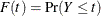 as the cumulative distribution function of Y. For
  , the pth quantile of the population cumulative distribution function is
![\[ Q(p)=\inf \{ y: F(y)\ge p\} \]](images/statug_surveymeans0105.png)
Estimate of Quantile
Let  be the observed values for variable Y that are associated with sampling weights, where
  are the stratum index, cluster index, and member index, respectively, as shown in the section Definitions and Notation. Let
 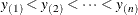 denote the sample order statistics for variable Y.
An estimate of quantile  is
is
![\[ \hat Q(p)= \left\{ \begin{array}{ll} y_{(1)} & \mbox{ if } p<\hat F(y_{(1)}) \\ y_{(k)}+\displaystyle {\frac{p-\hat F(y_{(k)})}{\hat F(y_{(k+1)})-\hat F(y_{(k)})}} (y_{(k+1)}-y_{(k)}) & \mbox{ if } \hat F(y_{(k)}) \le p < \hat F(y_{(k+1)}) \\ y_{(n)} & \mbox{ if } p=1 \end{array} \right. \]](images/statug_surveymeans0110.png)
where  is the estimated cumulative distribution for Y,
![\[ \hat F(t)=\frac{\sum _{h=1}^ H\sum _{i=1}^{n_ h} \sum _{j=1}^{m_{hi}}w_{hij}I(y_{hij}\le t)}{\sum _{h=1}^ H\sum _{i=1}^{n_ h}\sum _{j=1}^{m_{hi}}w_{hij}} \]](images/statug_surveymeans0112.png)
and  is the indicator function.
Standard Error
How PROC SURVEYMEANS estimates the standard error of a quantile depends on which variance method you specify in the VARMETHOD= option.
Taylor Series Method
When you specify VARMETHOD=TAYLOR
, or by default if you do not specify the VARMETHOD= option, PROC SURVEYMEANS uses Woodruff’s method (Dorfman and Valliant
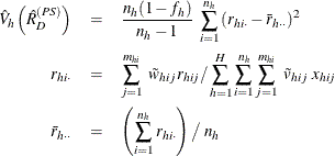
1993; Särndal, Swensson, and Wretman 1992; Francisco and Fuller 1991) to estimate the variances of quantiles. This method first constructs a confidence interval on a quantile  . Then it uses the width of the confidence interval to estimate the standard error of . To construct the confidence interval, PROC SURVEYMEANS first estimates the variance of the estimated distribution function
 by
by
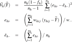
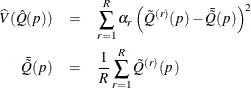
![\[ \hat V(\hat F(\hat Q(p))) =\sum _{h=1}^ H \frac{n_ h(1-f_ h)}{n_ h-1} ~ \sum _{i=1}^{n_ h} {(e_{hi\cdot }-\bar{e}_{h\cdot \cdot })^2} \]](images/statug_surveymeans0116.png)
where
Then % confidence limits for can be constructed by
![\[ \left(\hat p_ L, \, \, \, \, \, \, \hat p_ U\right)=\left(\hat F(\hat Q(p))-t_{\mi{df},\, \, \alpha /2}\sqrt {\hat V(\hat F(\hat Q(p)))}, \, \, \, \, \, \, \, \, \hat F(\hat Q(p))+t_{\mi{df},\, \, \alpha /2}\sqrt {\hat V(\hat F(\hat Q(p)))}\right) \]](images/statug_surveymeans0118.png)
where is the th percentile of the t distribution with df degrees of freedom, described in the section Degrees of Freedom.
When  is out of the range of [0,1], the procedure does not compute the standard error of .
The  th quantile is defined as
![\[ \hat Q(\hat p_ L)= \left\{ \begin{array}{ll} y_{(1)} & \mbox{ if } \hat p_ L<\hat F(y_{(1)}) \\ y_{(k_ L)}+\displaystyle {\frac{\hat p_ L-\hat F(y_{(k_ L)})}{\hat F(y_{(k_ L+1)})-\hat F(y_{(k_ L)})}} (y_{(k_ L+1)}-y_{(k_ L)}) & \mbox{ if } \hat F(y_{(k_ L)}) \le \hat p_ L < \hat F(y_{(k_ L+1)}) \\ y_{(d)} & \mbox{ if } \hat p_ L=1 \end{array} \right. \]](images/statug_surveymeans0121.png)
and the  th quantile is defined as
![\[ \hat Q(\hat p_ U)= \left\{ \begin{array}{ll} y_{(1)} & \mbox{ if } \hat p_ U<\hat F(y_{(1)}) \\ y_{(k_ U)}+\displaystyle {\frac{\hat p_ U-\hat F(y_{(k_ U)})}{\hat F(y_{(k_ U+1)})-\hat F(y_{(k_ U)})}} (y_{(k_ U+1)}-y_{(k_ U)}) & \mbox{ if } \hat F(y_{(k_ U)}) \le \hat p_ U < \hat F(y_{(k_ U+1)}) \\ y_{(d)} & \mbox{ if } \hat p_ U=1 \end{array} \right. \]](images/statug_surveymeans0123.png)
The standard error of is then estimated by
![\[ \hat{\mbox{StdErr}}(\hat Q(p)) = \frac{\hat Q(\hat p_ U) - \hat Q(\hat p_ L)}{2t_{\mi{df},\, \, \alpha /2}} \]](images/statug_surveymeans0124.png)
where is the th percentile of the t distribution with df degrees of freedom.
Replication Methods
When you use the jackknife replication method as described in the section Replication Methods for Variance Estimation, the following naive replication variance estimate for a quantile can have poor properties:
![\[ \widehat{V}(\hat Q(p)) = \sum _{r=1}^ R \alpha _ r \left( \hat Q^{(r)}(p) - {\hat Q(p)} \right)^2 \]](images/statug_surveymeans0125.png)
Here  is a coefficient that corresponds to each replicate, R is the number of replicates, and
  is the estimated quantile in the rth replicate.
Fuller (2009) proposes using a smoothing method similar to the following to modify the quantile estimates for each replicate before using this naive variance estimate for a quantile .
In the rth replicate ( ), denote
  to be the observed values of variable Y that are associated with the replicate weights. Let
 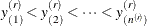 be the sample order statistics for variable Y in the rth replicate, where
  is the total number of observations whose replicate weights
  .
.
Let be the estimated pth quantile and  be the estimated cumulative distribution for Y,
![\[ \hat Q^{(r)}(p)= \left\{ \begin{array}{ll} y^{(r)}_{(1)} & \mbox{ if } p<\hat F^{(r)}(y^{(r)}_{(1)}) \\ y^{(r)}_{(k)}+\displaystyle {\frac{p-\hat F^{(r)}(y^{(r)}_{(k)})}{\hat F^{(r)}(y^{(r)}_{(k+1)})-\hat F^{(r)}(y^{(r)}_{(k)})}} (y^{(r)}_{(k+1)}-y^{(r)}_{(k)}) & \mbox{ if } \hat F^{(r)}(y^{(r)}_{(k)}) \le p < \hat F^{(r)}(y^{(r)}_{(k+1)}) \\ y^{(r)}_{(n^{(r)})} & \mbox{ if } p=1 \end{array} \right. \]](images/statug_surveymeans0134.png)
and
![\[ \hat F^{(r)}(t)=\frac{\sum _{h=1}^ H\sum _{i=1}^{n_ h} \sum _{j=1}^{m_{hi}}w^{(r)}_{hij}I(y^{(r)}_{hij}\le t)}{\sum _{h=1}^ H\sum _{i=1}^{n_ h}\sum _{j=1}^{m_{hi}}w^{(r)}_{hij}} \]](images/statug_surveymeans0135.png)
where is the indicator function.
Choose a segment in the distribution function by two points,  and
and  ,
,
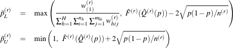
where  is the replicate weight that corresponds to
  in the rth replicate. Then a modified pth quantile in the rth replicate is defined by
![\[ \tilde Q^{(r)}(p) = \hat Q^{(r)}(\tilde p^{(r)}_ L) + \displaystyle {\frac{\hat Q^{(r)}(\tilde p^{(r)}_ U)-\hat Q^{(r)}(\tilde p^{(r)}_ L)}{\tilde p^{(r)}_ U-\tilde p^{(r)}_ L}} \left( {p-\tilde p^{(r)}_ L} \right) \]](images/statug_surveymeans0141.png)
PROC SURVEYMEANS then uses  as the quantile estimate in the rth replicate and its deviation from the mean of to estimate the variance of :
If you want to use the naive replication variance estimates by using instead of the smoothed to estimate the variance of , which are the default estimates before SAS/STAT 14.1, you can specify the method-option NAIVEQVAR as VARMETHOD=BRR(NAIVEQVAR)
or VARMETHOD=JACKKNIFE(NAIVEQVAR)
.
Confidence Limits
Symmetric % confidence limits are computed as
![\[ \left( \hat Q(p) - \hat{\mbox{StdErr}}(\hat Q(p)) ~ t_{\mi{df},\, \, \alpha /2} , \, \, \, \, \, \, \hat Q(p) + \hat{\mbox{StdErr}}(\hat Q(p)) ~ t_{\mi{df},\, \, \alpha /2} \right) \]](images/statug_surveymeans0144.png)
If you specify the NONSYMCL
option in the PROC SURVEYMEANS statement, when you use the VARMETHOD=TAYLOR
option, the procedure computes % nonsymmetric confidence limits:
![\[ \left(\hat Q(\hat p_ L), \, \, \, \, \, \hat Q(\hat p_ U) \right) \]](images/statug_surveymeans0145.png)
Quantile Estimation with Poststratification
When you specify a POSTSTRATA statement, the quantile estimation and its variance estimation incorporate poststratification. For more information about poststratification, see the section Poststratification.
For a selected sample, let be the poststratum index; let  be the population totals for each corresponding poststratum, and let
  be the indicator variable for the poststratum r that is defined by
![\[ I_{r}(h,i,j) = \left\{ \begin{array}{ll} 1 & \mbox{if observation } (h,i,j) \mbox{ belongs to the } r\mbox{th poststratum} \\ 0 & \mbox{otherwise} \end{array} \right. \]](images/statug_surveymeans0148.png)
Denote the total sum of original weights in the sample for each poststratum as
![\[ \psi _ r = \sum _{h=1}^ H\sum _{i=1}^{n_ h}\sum _{j=1}^{m_{hi}} ~ w_{hij} I_{r}(h,i,j) \]](images/statug_surveymeans0149.png)
Assume that the observation (h, i, j) belongs to the rth poststratum. Then the poststratification weight for the observation (h, i, j) is
![\[ \tilde{w}_{hij} = w_{hij} \frac{Z_ r}{\psi _ r} \]](images/statug_surveymeans0150.png)
Then the estimated cumulative distribution function of Y, and the estimated pth quantile estimation can be computed as in the section Estimate of Quantile by replacing the original weights, , with the poststratification weights,  .
.
When you specify VARMETHOD=TAYLOR
(or by default), the variance of is estimated as in the section Standard Error, except that the variance of the estimated distribution function is computed as follows.
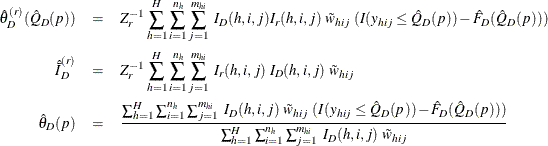
For each poststratum  , define
![\[ {\hat{\theta }}^{(r)}(\hat Q(p))= Z_ r^{-1} \sum _{h=1}^ H\sum _{i=1}^{n_ h} \sum _{j=1}^{m_{hi}} ~ I_{r}(h,i,j) ~ \tilde{w}_{hij} ~ (I(y_{hij} \le \hat Q(p)) - \hat F(\hat Q(p))) \]](images/statug_surveymeans0153.png)
where is the indicator function.
Assume that the observation (h, i, j) belongs to the rth poststratum. Let
![\[ \tilde{y}_{hij}=I(y_{hij} \le \hat Q(p)) - \hat F(\hat Q(p)) - {\hat{\theta }}^{(r)}(\hat Q(p)) \]](images/statug_surveymeans0154.png)
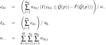
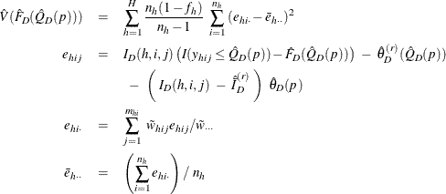
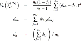
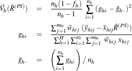
PROC SURVEYMEANS estimates the variance of the estimated distribution function with poststratification by
![\[ \hat V(\hat F(\hat Q(p))) =\sum _{h=1}^ H \frac{n_ h(1-f_ h)}{n_ h-1} ~ \sum _{i=1}^{n_ h} {(u_{hi\cdot }-\bar{u}_{h\cdot \cdot })^2} \]](images/statug_surveymeans0155.png)
where
Domain Quantile
Let Y be the variable of interest in a complex survey, and let a subpopulation of interest be domain D. Denote  as the cumulative distribution function of Y in domain D. For , the pth quantile of the population cumulative distribution function is
![\[ Q_ D(p)=\inf \{ y: F_ D(y)\ge p\} \]](images/statug_surveymeans0158.png)
Let be the corresponding indicator variable:
Assume that there are a total of d observations among the n observations in the entire sample that belong to domain D. Let 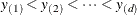 denote the order statistics of variable Y for these d observations that fall in domain D.
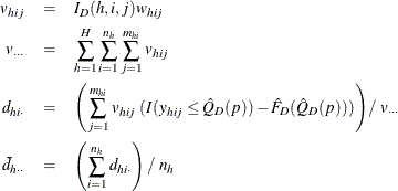
The cumulative distribution function of Y in domain D is estimated by
![\[ \hat F_ D(t)=\frac{\sum _{h=1}^ H\sum _{i=1}^{n_ h} \sum _{j=1}^{m_{hi}}w_{hij}I(y_{hij}\le t)I_{D}(h,i,j)}{\sum _{h=1}^ H\sum _{i=1}^{n_ h}\sum _{j=1}^{m_{hi}}w_{hij}I_{D}(h,i,j)} \]](images/statug_surveymeans0160.png)
and is the indicator function. Then the estimated quantile in domain D is
![\[ \hat Q_ D(p)= \left\{ \begin{array}{ll} y_{(1)} & \mbox{ if } p<\hat F_ D(y_{(1)}) \\ y_{(k)}+\displaystyle {\frac{p-\hat F_ D(y_{(k)})}{\hat F_ D(y_{(k+1)})-\hat F_ D(y_{(k)})}} (y_{(k+1)}-y_{(k)}) & \mbox{ if } \hat F_ D(y_{(k)}) \le p < \hat F_ D(y_{(k+1)}) \\ y_{(d)} & \mbox{ if } p=1 \end{array} \right. \]](images/statug_surveymeans0161.png)
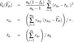
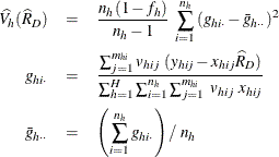
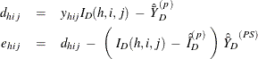
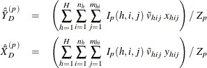
In order to estimate the variance for  , PROC SURVEYMEANS first estimates the variance of the estimated distribution function
  in domain D. When you specify VARMETHOD=TAYLOR
(or by default), the variance of is estimated by
in domain D. When you specify VARMETHOD=TAYLOR
(or by default), the variance of is estimated by
![\[ \hat V(\hat F_ D(\hat Q_ D(p))) =\sum _{h=1}^ H \frac{n_ h(1-f_ h)}{n_ h-1} ~ \sum _{i=1}^{n_ h} {(d_{hi\cdot }-\bar{d}_{h\cdot \cdot })^2} \]](images/statug_surveymeans0164.png)
where
Then % confidence limits for can be constructed by  , where
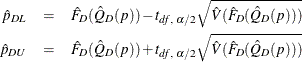
and is the th percentile of the t distribution with df degrees of freedom, described in the section Degrees of Freedom. When is out of the range of [0,1], PROC SURVEYMEANS does not compute the standard error of .
The  th quantile is then estimated as
![\[ \hat Q_ D(\hat{p}_{DL})= \left\{ \begin{array}{ll} y_{(1)} & \mbox{ if } \hat{p}_{DL}<\hat F_ D(y_{(1)}) \\ y_{(k_ L)}+\displaystyle {\frac{(\hat{p}_{DL}-\hat F_ D(y_{(k_ L)}))(y_{(k_ L+1)}-y_{(k_ L)})}{\hat F_ D(y_{(k_ L+1)})-\hat F_ D(y_{(k_ L)})}} & \mbox{ if } \hat F_ D(y_{(k_ L)}) \le \hat p_{DL} < \hat F_ D(y_{(k_ L+1)}) \\ y_{(d)} & \mbox{ if } \hat p_{DL}=1 \end{array} \right. \]](images/statug_surveymeans0169.png)
The  th quantile is then estimated as
![\[ \hat Q_ D(\hat{p}_{DU})= \left\{ \begin{array}{ll} y_{(1)} & \mbox{ if } \hat{p}_{DU}<\hat F_ D(y_{(1)}) \\ y_{(k_ U)}+\displaystyle {\frac{(\hat{p}_{DU}-\hat F_ D(y_{(k_ U)}))(y_{(k_ U+1)}-y_{(k_ U)})}{\hat F_ D(y_{(k_ U+1)})-\hat F_ D(y_{(k_ U)})}} & \mbox{ if } \hat F_ D(y_{(k_ U)}) \le \hat p_{DU} < \hat F_ D(y_{(k_ U+1)}) \\ y_{(d)} & \mbox{ if } \hat p_{DU}=1 \end{array} \right. \]](images/statug_surveymeans0171.png)
The standard error of is then estimated by
![\[ \hat{\mbox{StdErr}}(\hat Q_ D(p)) = \frac{\hat Q_ D(\hat{p}_{DU}) - \hat Q_ D(\hat{p}_{DL})}{2t_{\mi{df},\, \, \alpha /2}} \]](images/statug_surveymeans0172.png)
where is the th percentile of the t distribution with df degrees of freedom.
Symmetric % confidence limits for are computed as
![\[ \left( \hat Q_ D(p) - \hat{\mbox{StdErr}}(\hat Q_ D(p)) ~ t_{\mi{df},\, \, \alpha /2} , \, \, \, \, \, \, \hat Q_ D(p) + \hat{\mbox{StdErr}}(\hat Q_ D(p)) ~ t_{\mi{df},\, \, \alpha /2} \right) \]](images/statug_surveymeans0173.png)
If you specify the NONSYMCL
option in the PROC SURVEYMEANS statement, the procedure displays % nonsymmetric confidence limits as
![\[ \left(\hat Q_ D(\hat{p}_{DL}), \, \, \, \, \, \hat Q_ D(\hat{p}_{DU}) \right) \]](images/statug_surveymeans0174.png)
Domain Quantile Estimation with Poststratification
When you specify both a POSTSTRATA statement and a DOMAIN statement, the domain quantile estimation and its variance estimation incorporate poststratification. For more information about poststratification, see the section Poststratification.
For a selected sample, let be the poststratum index, let be the population totals for each corresponding poststratum, and let be the indicator variable for the poststratum r:
The poststratification weights, , are defined as in the section Quantile Estimation with Poststratification.
For domain D, let be the corresponding indicator variable:
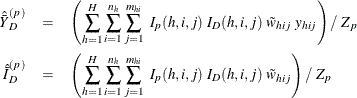
With poststratification, for variable Y, the estimated cumulative distribution in domain D,  , and its pth quantile estimation, , can be computed as in the section Domain Quantile by replacing the original weights, , with the poststratification weights, . However, the variance of , which is described in the section Domain Quantile, is computed as follows when you specify the VARMETHOD=TAYLOR
option (or by default).
, and its pth quantile estimation, , can be computed as in the section Domain Quantile by replacing the original weights, , with the poststratification weights, . However, the variance of , which is described in the section Domain Quantile, is computed as follows when you specify the VARMETHOD=TAYLOR
option (or by default).
Define
Assume that the observation (h, i, j) belongs to the rth poststratum. Then the variance of is estimated by
Geometric Mean
For a continuous variable Y that has positive values, the SURVEYMEANS procedure can compute its geometric mean and associated standard error and confidence limits. To request these statistics, you can specify statistic-keywords such as GEOMEAN, GMSTDERR, and GMCLM.
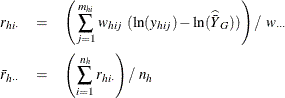
The geometric mean of Y from a sample is computed as
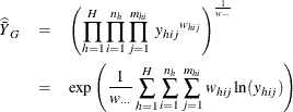
where
![\[ w_{\cdot \cdot \cdot } = \sum _{h=1}^ H\sum _{i=1}^{n_ h}\sum _{j=1}^{m_{hi}}w_{hij} \]](images/statug_surveymeans0179.png)
is the sum of the weights over all observations in the data set.
When you use the Taylor series method, the variance estimation for the geometric mean is computed as
where
The standard error of the geometric mean is the square root of the estimated variance:
![\[ \mbox{StdErr}(\widehat{{\bar{Y_ G}}})= \sqrt {\hat{V}(\widehat{\bar{Y}}_ G)} \]](images/statug_surveymeans0182.png)
The confidence limits for the geometric means are computed based on the confidence limits for the log transformation of the Y variable as
![\[ \left( \exp ( \ln (\widehat{\bar{Y}}_ G) ~ - ~ \gamma ), ~ ~ ~ ~ \exp ( \ln (\widehat{\bar{Y}}_ G) ~ + ~ \gamma ) \right) \]](images/statug_surveymeans0183.png)
where
![\[ \gamma = t_{\mi{df},\, \, \alpha /2} * \mbox{StdErr}(\widehat{{\bar{Y_ G}}}) / \widehat{\bar{Y}}_ G \]](images/statug_surveymeans0184.png)
and is the th percentile of the t distribution, with df calculated as in the section t Test for the Mean.
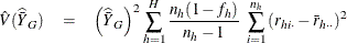
If you use replication methods to estimate the variance by specifying VARMETHOD=BRR
or VARMETHOD=JACKKNIFE
, the procedure computes the variance of a geometric means  by using the variability among replicate estimates to estimate the overall variance. See the section Replication Methods for Variance Estimation for more information.
Then the standard error is the square root of the estimated variance:
![\[ \mbox{StdErr}_ R(\widehat{{\bar{Y_ G}}})= \sqrt {\hat{V_ R}(\widehat{\bar{Y}}_ G)} \]](images/statug_surveymeans0186.png)
The confidence limits for the geometric means are computed based on the confidence limits for the log transformation of the variable Y as
![\[ \left( \exp ( \ln (\widehat{\bar{Y}}_ G) ~ - ~ \lambda ), ~ ~ ~ ~ \exp ( \ln (\widehat{\bar{Y}}_ G) ~ + ~ \lambda ) \right) \]](images/statug_surveymeans0187.png)
where
![\[ \lambda = t_{\mi{df},\, \, \alpha /2} * \mbox{StdErr}_ R (\widehat{{\bar{Y_ G}}}) / \widehat{{\bar{Y_ G}}} \]](images/statug_surveymeans0188.png)
and is the th percentile of the t distribution, with df calculated as in the section t Test for the Mean.
Poststratification
After a probability sample is drawn and survey data are collected, researchers sometimes want to stratify the sample according to auxiliary information about the sampled population. This process is often called poststratification.
When poststratification is done properly, it can improve efficiency. It can also be used to adjust the sampling weights such that the marginal distribution of the sampling weights is in agreement with known auxiliary information from other resources, such as the census. The adjusted weight is often called the poststratification weight. It is quite common for researchers to use poststratification techniques in survey data analysis.
Poststratification is also used by epidemiologists, who frequently analyze health survey data. They often compute statistics based on a process called direct standardization, a form of poststratification. For example, certain diseases, such as cancer, are more common among older populations. Therefore, to compare the prevalence rates among geographic regions that are populated with different age groups, it is necessary to make adjustments according to such demographic categories and to compute relative prevalence rates of the diseases.
For more information about poststratification, see Fuller (2009); Lohr (2010); Wolter (2007); Rao, Yung, and Hidiroglou (2002).
After you provide the population controls for each poststratum that is defined by the poststratification variables, the SURVEYMEANS procedure creates the poststratification weights accordingly. Then the procedure computes statistics that you request by using poststratification weights.
You can save the poststratification weights in an OUTPSWGT= data set to be used in subsequent analyses.
For a selected sample, let be the poststratum index; let  be the population totals for the corresponding poststrata; and let
  be a corresponding indicator variable for poststratum p defined by
![\[ I_{p}(h,i,j) = \left\{ \begin{array}{ll} 1 & \mbox{if observation }(h,i,j)\mbox{ belongs to poststratum} p \\ 0 & \mbox{otherwise} \end{array} \right. \]](images/statug_surveymeans0191.png)
Denote the total sum of original weights in the sample for each poststratum as
![\[ \psi _ p = \sum _{h=1}^ H\sum _{i=1}^{n_ h}\sum _{j=1}^{m_{hi}} ~ w_{hij} I_{p}(h,i,j) \]](images/statug_surveymeans0192.png)
Then the poststratification weight for observation (h, i, j) is
![\[ \tilde{w}_{hij} = w_{hij} \frac{Z_ p}{\psi _ p} \]](images/statug_surveymeans0193.png)
The SURVEYMEANS procedure computes statistics by using the poststratification weights instead of the original weights .
The standard error and confidence intervals of computed statistics are based on the estimated variances, which are computed by using either a replication method or the Taylor series method.
Replication Methods
When you specify VARMETHOD=BRR or VARMETHOD=JACKKNIFE , PROC SURVEYMEANS computes the variance of a statistic by using replication methods, as described in the section Replication Methods for Variance Estimation. However, with poststratification, an extra step is needed to adjust the weights.
First, PROC SURVEYMEANS constructs a replicate and computes appropriate replicate weights for the replicate. Then, by using the poststratification control totals, the procedure adjusts these replicate weights in the same way as described previously for constructing the poststratification weights for the full sample. Finally, PROC SURVEYMEANS computes the estimate for a desired statistics by using the poststratification weights that are adjusted from the replicate weights in the current replicate. Then the final variance is estimated by the variability among replicate estimates, as described in the section Replication Methods for Variance Estimation.
Taylor Series Method
When you specify VARMETHOD=TAYLOR , or by default when you do not specify the VARMETHOD= option, PROC SURVEYMEANS uses the Taylor series method to estimate the variances of requested statistics.
Variance of the Mean and Sum
The sum and mean of variable Y under poststratification are
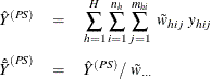
where
![\[ \tilde{w}_{\cdot \cdot \cdot } = \sum _{h=1}^ H\sum _{i=1}^{n_ h} \sum _{j=1}^{m_{hi}} \tilde{w}_{hij} \]](images/statug_surveymeans0195.png)
is the sum of the poststratification weights over all observations in the sample.
For each poststratum , let the mean of variable Y be
![\[ {\hat{\bar{Y}}}^{(p)} = \left( \sum _{h=1}^ H\sum _{i=1}^{n_ h} \sum _{j=1}^{m_{hi}} ~ I_{p}(h,i,j) ~ \tilde{w}_{hij} ~ y_{hij} \right) / ~ Z_ p \]](images/statug_surveymeans0196.png)
where  is the total of the poststratification weights in poststratum p.
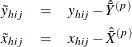
For observation (h, i, j), assume that it belongs to the pth poststratum. Let
![\[ \tilde{y}_{hij}=y_{hij}- \hat{\bar{Y}}^{(p)} \]](images/statug_surveymeans0198.png)
PROC SURVEYMEANS estimates the variance of  as
as
![\[ \hat{V}\left({\hat{\bar{Y}}}^{(PS)}\right) =\sum _{h=1}^ H {\hat{V}_ h \left({\hat{\bar{Y}}}^{(PS)}\right)} \]](images/statug_surveymeans0200.png)
where, if , then
and if , then
![\[ \hat{V}_ h \left({\hat{\bar{Y}}}^{(PS)}\right) = \left\{ \begin{array}{ll} \mbox{missing} & \mbox{ if } n_{h'}=1 \mbox{ for } h’=1, 2, \ldots , H \\ 0 & \mbox{ if } n_{h'}>1 \mbox{ for some } 1 \le h’ \le H \end{array} \right. \]](images/statug_surveymeans0202.png)
PROC SURVEYMEANS estimates the variance of  as
as
![\[ \hat{V}_ h \left({\hat{{Y}}}^{(PS)}\right) = \hat{V}_ h \left({\hat{\bar{Y}}}^{(PS)}\right) ~ {\tilde{w}}_{\cdot \cdot \cdot }^2 \]](images/statug_surveymeans0204.png)
Variance of the Domain Mean and Sum
For a domain D, let be the corresponding indicator variable:
Let
![\[ \tilde{v}_{hij}= \tilde{w}_{hij}I_ D(h,i,j) = \left\{ \begin{array}{ll} \tilde{w}_{hij} & \mbox{if observation }(h,i,j)\mbox{ belongs to } D \\ 0 & \mbox{otherwise} \end{array} \right. \]](images/statug_surveymeans0205.png)
The sum and mean of variable Y under poststratification in domain D are
where
![\[ \tilde{v}_{\cdot \cdot \cdot } = \sum _{h=1}^ H\sum _{i=1}^{n_ h} \sum _{j=1}^{m_{hi}} \tilde{v}_{hij} \]](images/statug_surveymeans0207.png)
is the sum of the poststratification weights over all observations in the sample in domain D. For each poststratum , let the mean of variable Y and the mean of the domain indicator variable in each poststratum be
Assume that the observation (h, i, j) belongs to the pth poststratum. Let
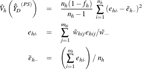
Then PROC SURVEYMEANS estimates the variance of domain sum  as
as
![\[ \hat{V}\left({\hat{{Y}}_ D}^{(PS)}\right) =\sum _{h=1}^ H {\hat{V}_ h \left({\hat{{Y}}_ D}^{(PS)}\right)} \]](images/statug_surveymeans0211.png)
where, if , then
and if , then
![\[ \hat{V}_ h \left({\hat{{Y}}_ D}^{(PS)}\right) = \left\{ \begin{array}{ll} \mbox{missing} & \mbox{ if } n_{h'}=1 \mbox{ for } h’=1, 2, \ldots , H \\ 0 & \mbox{ if } n_{h'}>1 \mbox{ for some } 1 \le h’ \le H \end{array} \right. \]](images/statug_surveymeans0213.png)
Then PROC SURVEYMEANS estimates the variance of domain mean  as
as
![\[ \hat{V}\left({\hat{\bar{Y}}_ D}^{(PS)}\right) =\sum _{h=1}^ H {\hat{V}_ h \left({\hat{\bar{Y}}_ D}^{(PS)}\right)} \]](images/statug_surveymeans0215.png)
where, if , then
and if , then
![\[ \hat{V}_ h \left({\hat{\bar{Y}}_ D}^{(PS)}\right) = \left\{ \begin{array}{ll} \mbox{missing} & \mbox{ if } n_{h'}=1 \mbox{ for } h’=1, 2, \ldots , H \\ 0 & \mbox{ if } n_{h'}>1 \mbox{ for some } 1 \le h’ \le H \end{array} \right. \]](images/statug_surveymeans0217.png)
Variance of the Ratio
Suppose you want to calculate the ratio of variable Y to variable X. Let and be the values of variable X and variable Y, respectively, for observation (h, i, j).
The ratio of Y to X after poststratification is
![\[ \hat{R}^{(PS)} = \frac{ \sum _{h=1}^ H\sum _{i=1}^{n_ h} \sum _{j=1}^{m_{hi}} ~ \tilde{w}_{hij} ~ y_{hij} }{ \sum _{h=1}^ H\sum _{i=1}^{n_ h} \sum _{j=1}^{m_{hi}} ~ \tilde{w}_{hij} ~ x_{hij} } \]](images/statug_surveymeans0218.png)
where is the poststratification weight for observation  .
.
Assume that the observation (h, i, j) belongs to the pth poststratum. Let
where  and
and  are the means of variable Y and variable X, respectively, in poststratum p.
The variance of  is estimated by
![\[ \hat{V}(\hat{R}^{(PS)}) = \sum _{h=1}^ H \hat{V_ h}(\hat{R}^{(PS)}) \]](images/statug_surveymeans0224.png)
where, if , then
and if , then
![\[ \hat{V_ h}(\hat{R}^{(PS)}) = \left\{ \begin{array}{ll} \mbox{missing} & \mbox{ if } n_{h'}=1 \mbox{ for } h’=1, 2, \ldots , H \\ 0 & \mbox{ if } n_{h'}>1 \mbox{ for some } 1 \le h’ \le H \end{array} \right. \]](images/statug_surveymeans0226.png)
Variance of the Domain Ratio
For a domain D, let be the corresponding indicator variable:
Let
The ratio of variable Y to variable X in domain D after poststratification is estimated by
![\[ {\hat{R}}_ D^{(PS)} = \frac{ \sum _{h=1}^ H\sum _{i=1}^{n_ h} \sum _{j=1}^{m_{hi}} ~ \tilde{w}_{hij} ~ y_{hij} ~ I_ D(h,i,j) }{ \sum _{h=1}^ H\sum _{i=1}^{n_ h} \sum _{j=1}^{m_{hi}} ~ \tilde{w}_{hij} ~ x_{hij} ~ I_ D(h,i,j) } \]](images/statug_surveymeans0227.png)
For each poststratum , let the mean of variable X and Y in each poststratum be
Assume that the observation (h, i, j) belongs to the pth poststratum. Let
![\[ r_{hij} = y_{hij}I_ D(h,i,j) ~ -~ {\hat{\bar{Y}}}_{D}^{(p)} ~ -~ \left( ~ x_{hij}I_ D(h,i,j) ~ -~ {\hat{\bar{X}}}_{D}^{(p)} ~ \right) ~ {\hat{R}}_ D^{(PS)} \]](images/statug_surveymeans0229.png)
Then PROC SURVEYMEANS estimates the variance of domain ratio  after poststratification as
![\[ \hat{V}\left({\hat{R}}_ D^{(PS)}\right) =\sum _{h=1}^ H {\hat{V}_ h \left({\hat{{R}}_ D}^{(PS)}\right)} \]](images/statug_surveymeans0231.png)
where, if , then
and if , then
![\[ \hat{V}_ h \left({\hat{R}}_ D^{(PS)}\right) = \left\{ \begin{array}{ll} \mbox{missing} & \mbox{ if } n_{h'}=1 \mbox{ for } h’=1, 2, \ldots , H \\ 0 & \mbox{ if } n_{h'}>1 \mbox{ for some } 1 \le h’ \le H \end{array} \right. \]](images/statug_surveymeans0233.png)