The SPP Procedure
-
Overview

- Getting Started
-
Syntax
-
DetailsTesting for Complete Spatial RandomnessExploring Interpoint InteractionDistance Functions for Multitype Point PatternsBorder Edge Correction for Distance FunctionsConfidence Intervals for Summary StatisticsRipley-Rasson Window EstimatorCovariate Dependence TestsNonparametric Intensity EstimationInhomogeneous Poisson Process Model FittingNegative Binomial ModelingOutput Data SetsDisplayed OutputODS Table NamesODS Graphics
-
Examples
- References
Getting Started: SPP Procedure
This example uses forestry data, which are shown in Figure 105.4, to show how you can use PROC SPP to fit a model for the first-order intensity of a spatial point pattern. The Sashelp.BEI data set contains the locations of 3,604 trees in tropical rain forests. A study window of 1,000  500 square kilometers is appropriate. The data set also contains covariates that are represented by the variables
 Gradient and Elevation, which are collected at 20,301 locations on a regular grid across the study region. The variable Trees distinguishes the event observations in the data set. These data are a part of a much larger data set, which contains the
positions of hundreds of thousands of trees that belong to thousands of species (Condit 1998; Hubbell and Foster 1983; Condit, Hubbell, and Foster 1996).[40] The Sashelp.BEI data set contains five variables:
-
XandY: the X and Y coordinates for locations of trees and for measurements of the height and slope of the study area -
Trees: a 0/1 variable that indicates which observation corresponds to locations of trees: 1 indicates the presence of a tree, and 0 indicates absence -
Elevation: which measures how far the study area is above sea level -
Gradient: which measures the slope of the study area
The following statements produce a plot of the event observations (which is shown in Figure 105.4) and plots of the covariates (which are shown in Figure 105.5 and Figure 105.6).
ods graphics on;
proc spp data=sashelp.bei plots(equate)=(trends observations);
   process trees = (x, y /area=(0,0,1000,500) Event=Trees);
   trend grad = field(x,y, gradient);
   trend elev = field(x,y, elevation);
run;
In addition, the preceding statements produce three tables, which are shown in Figure 105.1, Figure 105.2, and Figure 105.3. The number of observations in the combined data set is shown in Figure 105.1; it includes both the number of event observations and the number of covariate observations.
Figure 105.1: Number of Events and Number of Covariate Observations
Figure 105.2 provides some summary information about the point pattern, including the average intensity or the number of events per unit area.
Figure 105.2: Exploratory Information about the Point Pattern
| Summary of Point Pattern | |
|---|---|
| Data Type | Point Pattern |
| Pattern Name | trees |
| Region Type | User Defined Window |
| Region X Range | [0,1000] Units |
| Region Y Range | [0,500] Units |
| Region X Size | 1000 Units |
| Region Y Size | 500 Units |
| Region Area | 500000 Square Units |
| Observations in Window | 3604 |
| Average Intensity | 0.007208 |
| Grid Nodes in X | 50 |
| Grid Nodes in Y | 50 |
| Grid Nodes in Window | 2500 |
| Quadrat Dimension in X | 10 |
| Quadrat Dimension in Y | 10 |
Figure 105.3 provides the results of a default  quadrat-based Pearson chi-square test for CSR.
Figure 105.3: Pearson Chi-Square Test for CSR
Figure 105.4: Spatial Point Pattern of Tropical Rain forest Trees
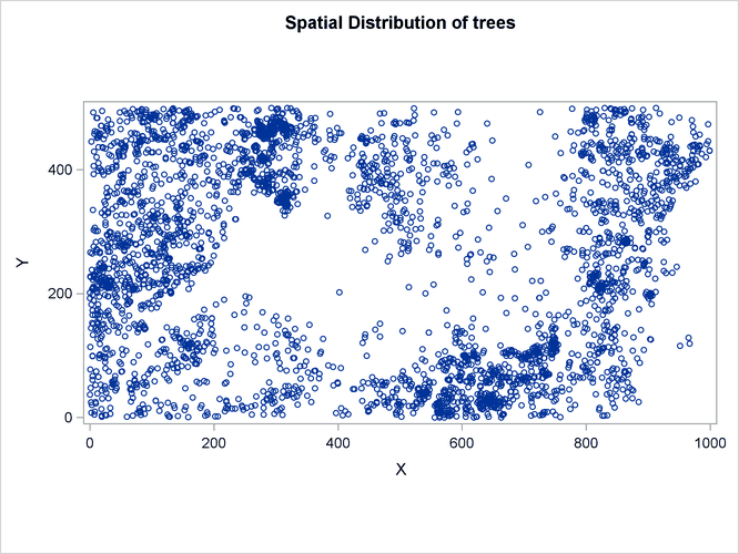
Figure 105.5: Spatial Covariate Gradient
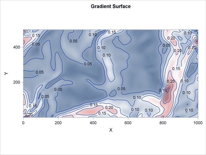
Figure 105.6: Spatial Covariate Elevation
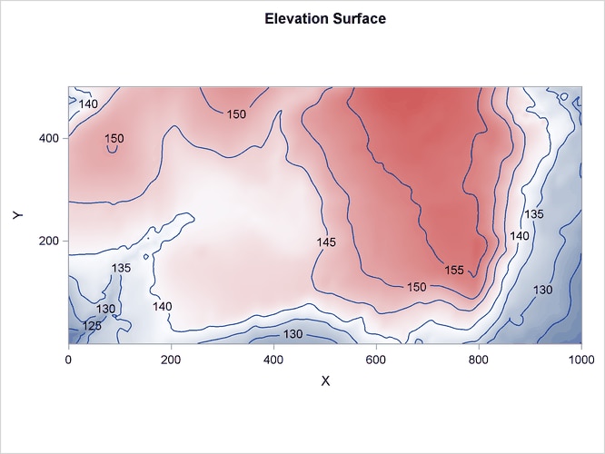
The variables Gradient and Elevation are both continuous functions, because any arbitrary point that is chosen in the study area has a value for both these variables.
However, these variables are sampled at select points where measuring them is easy. In spatial analysis and geographic information
systems (GISs), such variables are termed field variables and are associated with a spatial trend. You can include such variables in the SPP procedure by using the TREND
statement.
The sashelp.bei data contains combined information for both the point pattern and the spatial covariates. However, the SPP procedure requires
you to identify the point pattern event identifier separately. This is done by using the EVENT=
option in the PROCESS
statement to specify that the variable Trees identifies the event.
It is natural to suppose that tree growth is affected by the gradient and elevation of the surrounding land. Hence, you can
use the gradient and elevation in a parametric model to model the intensity of tree growth in the study area. Such a model
is an inhomogeneous Poisson process (Baddeley 2010, p. 354), whose first-order intensity,  , is log linear in the covariates. You can use the MODEL
statement to compose models for a point pattern’s intensity. In the MODEL
statement, you specify the response pattern on the left side. The response pattern is a process that you define before you
specify the MODEL
statement. You can specify any covariates that are likely to influence the target point pattern on the right side of the
MODEL
statement syntax.
, is log linear in the covariates. You can use the MODEL
statement to compose models for a point pattern’s intensity. In the MODEL
statement, you specify the response pattern on the left side. The response pattern is a process that you define before you
specify the MODEL
statement. You can specify any covariates that are likely to influence the target point pattern on the right side of the
MODEL
statement syntax.
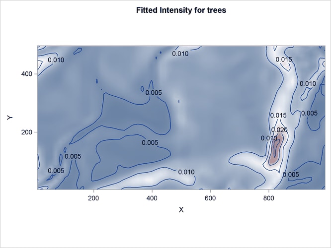
To obtain a plot of the model-based intensity estimate, you specify the PLOTS=INTENSITY
option. In addition, if you want to request residual diagnostics, you can specify the PLOTS=RESIDUAL
option. If you want to specify a response grid to obtain the intensity estimates, you can use the GRID
option in the MODEL
statement. The following statements explore the influence of the covariates Elevation and Gradient on the intensity of Tree presence:
proc spp data=sashelp.bei plots(equate)=(residual intensity);
   process trees = (x,y /area=(0,0,1000,500) event=Trees);
   trend elev = field(x,y,elevation);
   trend grad = field(x,y,gradient);
   model trees = elev grad / grid(64,64) residual(B=70) ;
run;
In addition to the tables shown in previous figures, these statements produce a table that contains the parameter estimates
(Figure 105.7) and a fit summary table (Figure 105.8). The parameter estimates designate the intercept value and the values of the factors of the model terms. The relative values
of the parameter estimates indicate how much each factor contributes to the model. In this case, Gradient is much more important in modeling where trees grow than Elevation, although both are highly significant.
Figure 105.7: Parameter Estimates Table
The fit summary table in Figure 105.8 shows the model fit statistics. You can use these values to compare multiple fits from different models and to select an optimal model in your study.
Figure 105.8: Fit Summary Table
The corresponding fitted intensity is shown in Figure 105.9.
Figure 105.9: Intensity Estimates of Tree presence in Study Area
The resulting residual diagnostics are shown in Figure 105.10.
Figure 105.10: Residual Diagnostics for Fitted Log-Intensity Model
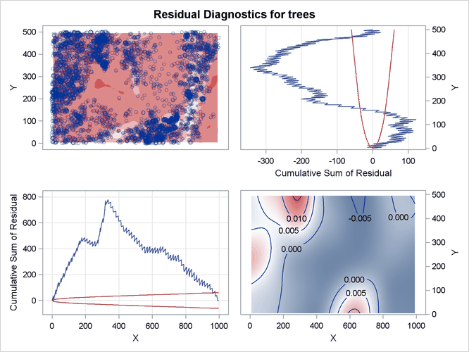
The residual diagnostics plot in Figure 105.10 provides an informal assessment of the fitted parametric model. In particular, the smoothed residual plot in the right bottom
corner reveals a trend in the residual that is not accounted for by the model. In addition, the lurking variable plots with
respect to the coordinate variables show significant deviation from the  limits, indicating that the model does not account for a variation in intensity with respect to these variables.
[40] This data set is used with kind permission from Professor S. Hubbell, with acknowledgment of the support of the Center for Tropical Forest Science of the Smithsonian Tropical Research Institute and the primary granting agencies that have supported the BCI plot. The BCI forest dynamics research project was made possible by National Science Foundation grants to Stephen P. Hubbell: DEB-0640386, DEB-0425651, DEB-0346488, DEB-0129874, DEB-00753102, DEB-9909347, DEB-9615226, DEB-9615226, DEB-9405933, DEB-9221033, DEB-9100058, DEB-8906869, DEB-8605042, DEB-8206992, DEB-7922197, support from the Center for Tropical Forest Science, the Smithsonian Tropical Research Institute, the John D. and Catherine T. MacArthur Foundation, the Mellon Foundation, the Small World Institute Fund, and numerous private individuals, and through the hard work of over 100 people from 10 countries over the past two decades. The plot project is part of the Center for Tropical Forest Science, a global network of large-scale demographic tree plots.