The SPP Procedure
-
Overview

- Getting Started
-
Syntax
-
DetailsTesting for Complete Spatial RandomnessExploring Interpoint InteractionDistance Functions for Multitype Point PatternsBorder Edge Correction for Distance FunctionsConfidence Intervals for Summary StatisticsRipley-Rasson Window EstimatorCovariate Dependence TestsNonparametric Intensity EstimationInhomogeneous Poisson Process Model FittingNegative Binomial ModelingOutput Data SetsDisplayed OutputODS Table NamesODS Graphics
-
Examples
- References
Example 105.3 Intensity Model Validation Diagnostics
Model validation diagnostics help you evaluate whether the fitted model that involves the covariates is appropriate for the specified point pattern. The SPP procedure provides two types of diagnostics:
-
goodness-of-fit test
-
residual diagnostics
This example demonstrates the usage of these diagnostics for model validation. It uses a simulated point pattern data set
and also simulates two covariates over a  grid. The following statements define functions for simulating a spatial point pattern given an intensity function by the
method of random thinning of Lewis and Shedler (1979), as discussed in Schabenberger and Gotway (2005) and Wicklin (2013). For more information about the method and the code, see Wicklin (2013). The functions are saved in a SAS/IML storage catalog to make them available for reuse.
grid. The following statements define functions for simulating a spatial point pattern given an intensity function by the
method of random thinning of Lewis and Shedler (1979), as discussed in Schabenberger and Gotway (2005) and Wicklin (2013). For more information about the method and the code, see Wicklin (2013). The functions are saved in a SAS/IML storage catalog to make them available for reuse.
ods graphics on;

proc iml;
   start Uniform2d(n, a, b);
      u = j(n, 2);
      call randgen(u, "Uniform");
      return( u # (a||b) );
   finish;

   start HomogPoissonProcess(lambda, a, b);
      n = 1;
      call randgen(n,"Poisson", lambda*2500);
      return( Uniform2d(n, a, b) );
   finish;

   start InhomogPoissonProcess(a, b) global(lambda0);
      u = HomogPoissonProcess(lambda0, a, b);
      lambda = Intensity(u[,1], u[,2]);
      r = shape(.,sum(lambda<=lambda0),1);
      call randgen(r,"Bernoulli", lambda[loc(lambda<=lambda0)]/lambda0);
      return( u[loc(r),] );
   finish;

   reset storage=sasuser.SPPThin;
   store module=Uniform2d
         module=HomogPoissonProcess
         module=InhomogPoissonProcess;
quit;
The following statements define a certain intensity function that is based on the elevation and slope of the land around particular
hills, with hills characterized by a four-column matrix Hills, where the first two columns give the X and Y coordinates of each hill center and the last two columns give their height
and radii. In the model, both elevation and slope are assumed to be positive, with a negative effect on intensity, so lambda0
(the maximum value of intensity) is the value at Elevation=Slope=0.
proc iml;
   %let xH = Hills[iHill,1];
   %let yH = Hills[iHill,2];
   %let hH = Hills[iHill,3];
   %let rH = Hills[iHill,4];

   start Elevation(x,y) global(Hills);
      Elevation = 0;
      do iHill = 1 to nrow(Hills);
         Height = &hH*exp(-((x - &xH)##2 + (y - &yH)##2)/&rH);
         Elevation = Elevation + Height;
      end;
      return(Elevation);
   finish;

   start Slope(x,y) global(Hills);
      xslope = 0;
      yslope = 0;
      do iHill = 1 to nrow(Hills);
         Height = &hH*exp(-((x - &xH)##2 + (y - &yH)##2)/&rH);
         dxHeight = -2*Height#(x - &xH)/&rH;
         dyHeight = -2*Height#(y - &yH)/&rH;
         xslope   = xslope + dxHeight;
         yslope   = yslope + dyHeight;
      end;
      Slope = sqrt(xslope##2 + yslope##2);
      return(Slope);
   finish;

   start Intensity(x,y) global(lambda0);
      lin = 0.5 - 2*Elevation(x,y) - 10*Slope(x,y);
      return(exp(lin));
   finish;

   lambda0 = exp(0.5);

   reset storage=sasuser.SPPFlowers;
   store lambda0 module=Elevation module=Slope module=Intensity;
quit;
Finally, the following statements use the simulation method of Wicklin (2013) and the previously defined intensity to simulate a spatial point pattern on 10 hills in an area of  units. The covariates, Elevation and Slope, are also computed over a grid of points in the region of interest.
proc iml;
   reset storage=sasuser.SPPThin;
   load module=Uniform2d
        module=HomogPoissonProcess
        module=InhomogPoissonProcess;

   reset storage=sasuser.SPPFlowers;
   load  module=Elevation module=Slope module=Intensity lambda0;

   a = 50;
   b = 50;

   Hills = { 9.2 48.5 0.2 13.0,
           46.1 48.5 0.3 26.6,
            2.5  3.3 0.7 26.2,
           42.7  3.4 0.9 14.9,
           13.6 34.5 1.0 11.3,
           34.4 20.6 0.3 14.4,
           23.8 42.2 0.4 29.5,
           29.1 18.9 0.5 25.3,
           46.6 46.5 0.3 14.9,
           19.6 23.6 0.5  8.4};

   call randseed(12345);

   free Cov;
   Cov = j((a+1) * (b+1), 5, 0);
   do x = 0 to a; do y = 0 to b;
      Cov[x#(a+1)+y+1,] =  (x || y || Elevation(x,y) || Slope(x,y)
                           || Intensity(x,y));
   end; end;

   create Covariates var {"x" "y" "Elevation" "Slope" "Intensity"};
   append from Cov;
   close Covariates;

   Hills = Hills // {25 5 2 15};
   z = InhomogPoissonProcess(a, b);

   create Events var {"x" "y"};
   append from z;
   close;

quit;
data simAll;
   set Events(in=e) Covariates;
   Flowers = e;
run;
The point pattern data set and the covariate data set are combined in the simAll data set and the event observations can be identified by using a variable Flowers.
proc spp data=simAll plots(equate)=(trends observations);
   process trees = (x, y /area=(0,0,50,50) Event=Flowers);
   trend grad = field(x,y, Elevation);
   trend elev = field(x,y, Slope);
run;
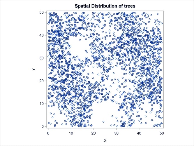
Output 105.3.1 shows the point pattern. The point pattern has been simulated to include a Gaussian bump at the center of the study region.
Output 105.3.1: Spatial Point Pattern of Simulated Flowers
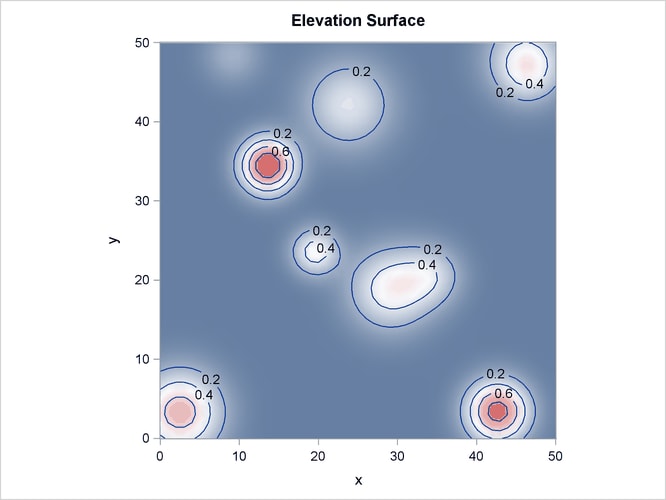
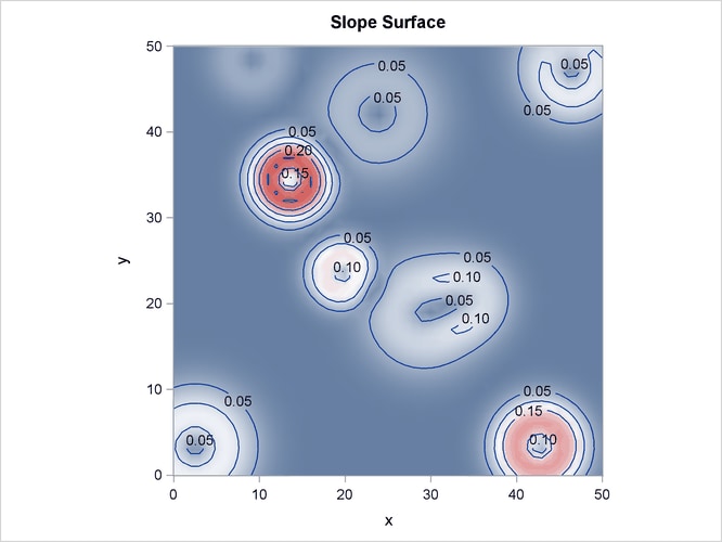
Output 105.3.2 shows the spatial covariate Elevation, and Output 105.3.3 shows the spatial covariate Slope. The covariates have been simulated to include several Gaussian hills, and they are continuous within the study region (that is, every point in the region has a value for these covariates).
Output 105.3.2: Spatial Covariate Elevation
Output 105.3.3: Spatial Covariate Slope
The following code fits an intensity model for the simulated point pattern that involves the simulated covariates Elevation and Slope. It also requests model validation diagnostics, including residuals and the goodness-of-fit test.
proc spp data=simAll seed=1  plots(equate)=(residual);
   process trees = (x,y /area=(0,0,50,50) Event=Flowers) /quadrat(4,2 /details);
   trend elev = field(x,y, Elevation);
   trend slope = field(x,y, Slope);
   model trees = elev slope/residual(b=5) gof;
run;
Output 105.3.4 shows the fitted intensity estimate that is based on the model that involves just the covariates Elevation and Slope.
Output 105.3.4: Fitted Intensity Estimate for the Simulated Point Pattern
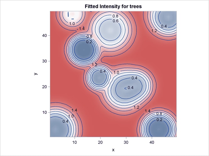
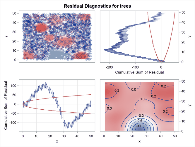
Output 105.3.5 shows the residual diagnostics for the model. It is clear from the smoothed residual plot at the bottom right corner of Output 105.3.5 that the model that involves just the covariates Elevation and Slope fails to account for the Gaussian bump in the middle of the study region. This is revealed by the trend at the center of
the smoothed residual plot at the bottom right corner of Output 105.3.5.
Output 105.3.5: Residual Diagnostics for the Fitted Model
Consequently, the goodness-of-fit test rejects the hypothesis that the point pattern was generated by the fitted model. This is evident in the low p-value that is obtained for the Pearson chi-square test for goodness of fit, which is shown in Output 105.3.6.
Output 105.3.6: Pearson Chi-Square Test for Goodness of Fit
Output 105.3.7 shows the corresponding Pearson residuals for the goodness-of-fit test.
Output 105.3.7: Quadrat Information and Pearson Residuals for Goodness-of-Fit Test
| Quadrat Information for Goodness-of-Fit Test |
|||||
|---|---|---|---|---|---|
| ID | Quadrat | Expected Frequency |
Count | Percentage | Pearson Residual |
| 1 | (1,1) | 352 | 375 | 13.58% | 1.20 |
| 2 | (2,1) | 398 | 310 | 11.22% | -4.41 |
| 3 | (3,1) | 298 | 184 | 6.66% | -6.60 |
| 4 | (4,1) | 323 | 349 | 12.64% | 1.45 |
| 5 | (1,2) | 383 | 450 | 16.29% | 3.43 |
| 6 | (2,2) | 261 | 264 | 9.56% | 0.19 |
| 7 | (3,2) | 383 | 397 | 14.37% | 0.70 |
| 8 | (4,2) | 371 | 433 | 15.68% | 3.22 |
When the model involves only the covariates Elevation and Slope, the residual diagnostics and the goodness-of-fit test both reveal discrepancies in the model that do not fully account for
the simulated point pattern. In particular, the model misses the Gaussian bump in the middle of the study region.